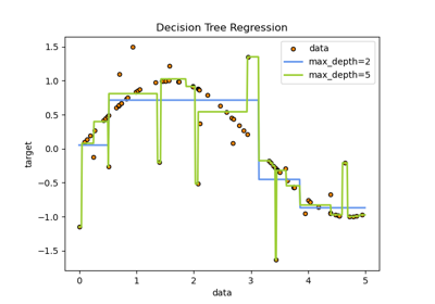
使用 KBinsDiscretizer 離散化連續特徵#

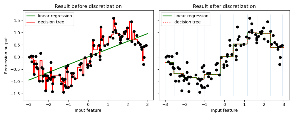
此範例比較使用和不使用實值特徵離散化時，線性迴歸（線性模型）和決策樹（基於樹的模型）的預測結果。

如離散化前的結果所示，線性模型建立速度快且相對容易解釋，但只能對線性關係進行建模，而決策樹可以建立更複雜的資料模型。在連續資料上使線性模型更強大的方法之一是使用離散化（也稱為分箱）。在此範例中，我們將特徵離散化並對轉換後的資料進行獨熱編碼。請注意，如果箱體不夠寬，則明顯會增加過擬合的風險，因此離散化器的參數通常應在交叉驗證下進行調整。

離散化後，線性迴歸和決策樹的預測完全相同。由於特徵在每個箱體內都是恆定的，因此任何模型都必須預測箱體內所有點的相同值。與離散化前的結果相比，線性模型變得更具彈性，而決策樹則變得不那麼彈性。請注意，分箱特徵通常對基於樹的模型沒有任何好處，因為這些模型可以學習在任何地方分割資料。

Result before discretization, Result after discretization

# Authors: The scikit-learn developers
# SPDX-License-Identifier: BSD-3-Clause

import matplotlib.pyplot as plt
import numpy as np

from sklearn.linear_model import LinearRegression
from sklearn.preprocessing import KBinsDiscretizer
from sklearn.tree import DecisionTreeRegressor

# construct the dataset
rnd = np.random.RandomState(42)
X = rnd.uniform(-3, 3, size=100)
y = np.sin(X) + rnd.normal(size=len(X)) / 3
X = X.reshape(-1, 1)

# transform the dataset with KBinsDiscretizer
enc = KBinsDiscretizer(n_bins=10, encode="onehot")
X_binned = enc.fit_transform(X)

# predict with original dataset
fig, (ax1, ax2) = plt.subplots(ncols=2, sharey=True, figsize=(10, 4))
line = np.linspace(-3, 3, 1000, endpoint=False).reshape(-1, 1)
reg = LinearRegression().fit(X, y)
ax1.plot(line, reg.predict(line), linewidth=2, color="green", label="linear regression")
reg = DecisionTreeRegressor(min_samples_split=3, random_state=0).fit(X, y)
ax1.plot(line, reg.predict(line), linewidth=2, color="red", label="decision tree")
ax1.plot(X[:, 0], y, "o", c="k")
ax1.legend(loc="best")
ax1.set_ylabel("Regression output")
ax1.set_xlabel("Input feature")
ax1.set_title("Result before discretization")

# predict with transformed dataset
line_binned = enc.transform(line)
reg = LinearRegression().fit(X_binned, y)
ax2.plot(
    line,
    reg.predict(line_binned),
    linewidth=2,
    color="green",
    linestyle="-",
    label="linear regression",
)
reg = DecisionTreeRegressor(min_samples_split=3, random_state=0).fit(X_binned, y)
ax2.plot(
    line,
    reg.predict(line_binned),
    linewidth=2,
    color="red",
    linestyle=":",
    label="decision tree",
)
ax2.plot(X[:, 0], y, "o", c="k")
ax2.vlines(enc.bin_edges_[0], *plt.gca().get_ylim(), linewidth=1, alpha=0.2)
ax2.legend(loc="best")
ax2.set_xlabel("Input feature")
ax2.set_title("Result after discretization")

plt.tight_layout()
plt.show()