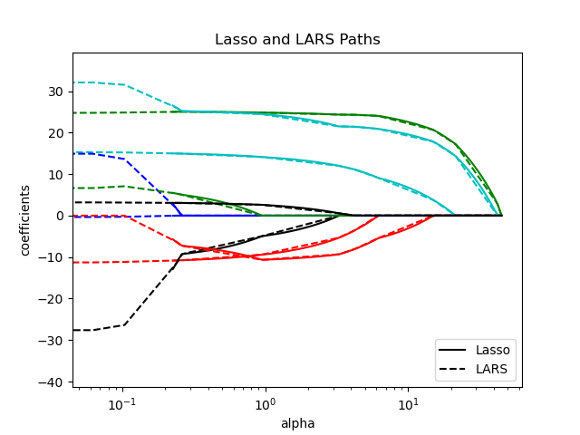
Lasso、Lasso-LARS 和彈性網路路徑#

此範例顯示如何計算沿著 Lasso、Lasso-LARS 和彈性網路正規化路徑的係數「路徑」。換句話說，它顯示了正規化參數 (alpha) 和係數之間的關係。

Lasso 和 Lasso-LARS 對係數施加稀疏性限制，鼓勵其中一些為零。彈性網路是 Lasso 的推廣，它將 L2 懲罰項添加到 L1 懲罰項。這允許一些係數為非零，同時仍然鼓勵稀疏性。

Lasso 和彈性網路使用坐標下降法計算路徑，而 Lasso-LARS 使用 LARS 演算法計算路徑。

路徑使用 lasso_path、lars_path 和 enet_path 計算。

結果顯示不同的比較圖

比較 Lasso 和 Lasso-LARS
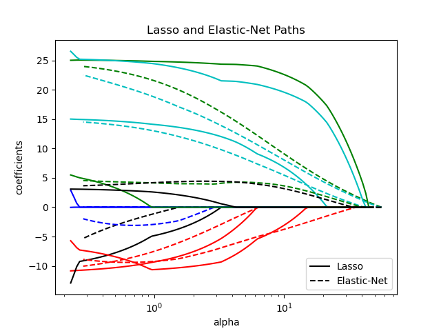
比較 Lasso 和彈性網路
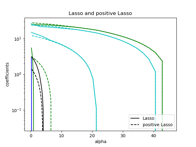
比較 Lasso 和正 Lasso
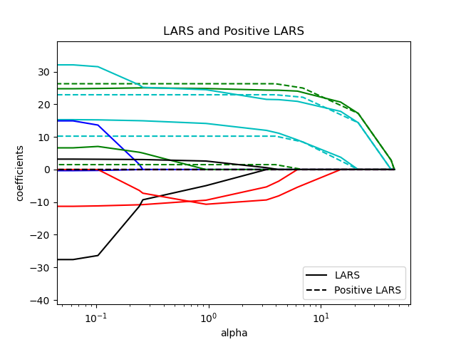
比較 LARS 和正 LARS
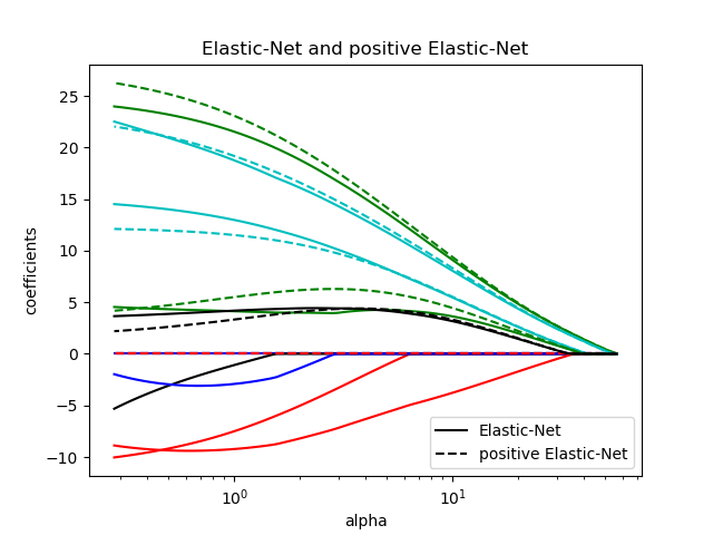
比較彈性網路和正彈性網路

每個圖都顯示了模型係數如何隨著正規化強度的變化而變化，提供了對這些模型在不同約束下行為的深入了解。

Computing regularization path using the lasso...
Computing regularization path using the positive lasso...
Computing regularization path using the LARS...
Computing regularization path using the positive LARS...
Computing regularization path using the elastic net...
Computing regularization path using the positive elastic net...

# Authors: The scikit-learn developers
# SPDX-License-Identifier: BSD-3-Clause

from itertools import cycle

import matplotlib.pyplot as plt

from sklearn.datasets import load_diabetes
from sklearn.linear_model import enet_path, lars_path, lasso_path

X, y = load_diabetes(return_X_y=True)
X /= X.std(axis=0)  # Standardize data (easier to set the l1_ratio parameter)

# Compute paths

eps = 5e-3  # the smaller it is the longer is the path

print("Computing regularization path using the lasso...")
alphas_lasso, coefs_lasso, _ = lasso_path(X, y, eps=eps)

print("Computing regularization path using the positive lasso...")
alphas_positive_lasso, coefs_positive_lasso, _ = lasso_path(
    X, y, eps=eps, positive=True
)

print("Computing regularization path using the LARS...")
alphas_lars, _, coefs_lars = lars_path(X, y, method="lasso")

print("Computing regularization path using the positive LARS...")
alphas_positive_lars, _, coefs_positive_lars = lars_path(
    X, y, method="lasso", positive=True
)

print("Computing regularization path using the elastic net...")
alphas_enet, coefs_enet, _ = enet_path(X, y, eps=eps, l1_ratio=0.8)

print("Computing regularization path using the positive elastic net...")
alphas_positive_enet, coefs_positive_enet, _ = enet_path(
    X, y, eps=eps, l1_ratio=0.8, positive=True
)

# Display results

plt.figure(1)
colors = cycle(["b", "r", "g", "c", "k"])
for coef_lasso, coef_lars, c in zip(coefs_lasso, coefs_lars, colors):
    l1 = plt.semilogx(alphas_lasso, coef_lasso, c=c)
    l2 = plt.semilogx(alphas_lars, coef_lars, linestyle="--", c=c)

plt.xlabel("alpha")
plt.ylabel("coefficients")
plt.title("Lasso and LARS Paths")
plt.legend((l1[-1], l2[-1]), ("Lasso", "LARS"), loc="lower right")
plt.axis("tight")

plt.figure(2)
colors = cycle(["b", "r", "g", "c", "k"])
for coef_l, coef_e, c in zip(coefs_lasso, coefs_enet, colors):
    l1 = plt.semilogx(alphas_lasso, coef_l, c=c)
    l2 = plt.semilogx(alphas_enet, coef_e, linestyle="--", c=c)

plt.xlabel("alpha")
plt.ylabel("coefficients")
plt.title("Lasso and Elastic-Net Paths")
plt.legend((l1[-1], l2[-1]), ("Lasso", "Elastic-Net"), loc="lower right")
plt.axis("tight")


plt.figure(3)
for coef_l, coef_pl, c in zip(coefs_lasso, coefs_positive_lasso, colors):
    l1 = plt.semilogy(alphas_lasso, coef_l, c=c)
    l2 = plt.semilogy(alphas_positive_lasso, coef_pl, linestyle="--", c=c)

plt.xlabel("alpha")
plt.ylabel("coefficients")
plt.title("Lasso and positive Lasso")
plt.legend((l1[-1], l2[-1]), ("Lasso", "positive Lasso"), loc="lower right")
plt.axis("tight")


plt.figure(4)
colors = cycle(["b", "r", "g", "c", "k"])
for coef_lars, coef_positive_lars, c in zip(coefs_lars, coefs_positive_lars, colors):
    l1 = plt.semilogx(alphas_lars, coef_lars, c=c)
    l2 = plt.semilogx(alphas_positive_lars, coef_positive_lars, linestyle="--", c=c)

plt.xlabel("alpha")
plt.ylabel("coefficients")
plt.title("LARS and Positive LARS")
plt.legend((l1[-1], l2[-1]), ("LARS", "Positive LARS"), loc="lower right")
plt.axis("tight")

plt.figure(5)
for coef_e, coef_pe, c in zip(coefs_enet, coefs_positive_enet, colors):
    l1 = plt.semilogx(alphas_enet, coef_e, c=c)
    l2 = plt.semilogx(alphas_positive_enet, coef_pe, linestyle="--", c=c)

plt.xlabel("alpha")
plt.ylabel("coefficients")
plt.title("Elastic-Net and positive Elastic-Net")
plt.legend((l1[-1], l2[-1]), ("Elastic-Net", "positive Elastic-Net"), loc="lower right")
plt.axis("tight")
plt.show()