注意
前往結尾以下載完整的範例程式碼。或透過 JupyterLite 或 Binder 在您的瀏覽器中執行此範例
理解決策樹結構#
可以分析決策樹結構,以進一步深入了解特徵與要預測的目標之間的關係。在此範例中,我們將展示如何檢索
二元樹結構;
每個節點的深度以及它是否為葉節點;
使用
decision_path方法的樣本到達的節點;使用 apply 方法的樣本到達的葉節點;
用於預測樣本的規則;
一組樣本共享的決策路徑。
# Authors: The scikit-learn developers
# SPDX-License-Identifier: BSD-3-Clause

import numpy as np
from matplotlib import pyplot as plt

from sklearn import tree
from sklearn.datasets import load_iris
from sklearn.model_selection import train_test_split
from sklearn.tree import DecisionTreeClassifier
訓練樹分類器#
首先,我們使用 DecisionTreeClassifier 來擬合 load_iris 資料集。
iris = load_iris()
X = iris.data
y = iris.target
X_train, X_test, y_train, y_test = train_test_split(X, y, random_state=0)

clf = DecisionTreeClassifier(max_leaf_nodes=3, random_state=0)
clf.fit(X_train, y_train)
樹結構#
決策分類器有一個名為 tree_ 的屬性,允許存取低階屬性,例如 node_count (節點總數) 和 max_depth (樹的最大深度)。tree_.compute_node_depths() 方法會計算樹中每個節點的深度。tree_ 也會儲存整個二元樹結構,表示為多個平行陣列。每個陣列的第 i 個元素會保存有關節點 i 的資訊。節點 0 是樹的根節點。某些陣列僅適用於葉節點或分割節點。在這種情況下,另一種類型的節點值是任意的。例如,陣列 feature 和 threshold 僅適用於分割節點。因此,這些陣列中葉節點的值是任意的。
在這些陣列中,我們有
children_left[i]:節點i的左子節點 ID,如果為葉節點,則為 -1children_right[i]:節點i的右子節點 ID,如果為葉節點,則為 -1feature[i]:用於分割節點i的特徵threshold[i]:節點i的閾值n_node_samples[i]:到達節點i的訓練樣本數impurity[i]:節點i的雜質weighted_n_node_samples[i]:到達節點i的加權訓練樣本數value[i, j, k]:到達節點 i 的訓練樣本摘要,適用於輸出 j 和類別 k (對於迴歸樹,類別設為 1)。有關value的詳細資訊,請參閱下方。
使用陣列,我們可以遍歷樹結構以計算各種屬性。下面,我們將計算每個節點的深度以及它是否為葉節點。
n_nodes = clf.tree_.node_count
children_left = clf.tree_.children_left
children_right = clf.tree_.children_right
feature = clf.tree_.feature
threshold = clf.tree_.threshold
values = clf.tree_.value

node_depth = np.zeros(shape=n_nodes, dtype=np.int64)
is_leaves = np.zeros(shape=n_nodes, dtype=bool)
stack = [(0, 0)]  # start with the root node id (0) and its depth (0)
while len(stack) > 0:
    # `pop` ensures each node is only visited once
    node_id, depth = stack.pop()
    node_depth[node_id] = depth

    # If the left and right child of a node is not the same we have a split
    # node
    is_split_node = children_left[node_id] != children_right[node_id]
    # If a split node, append left and right children and depth to `stack`
    # so we can loop through them
    if is_split_node:
        stack.append((children_left[node_id], depth + 1))
        stack.append((children_right[node_id], depth + 1))
    else:
        is_leaves[node_id] = True

print(
    "The binary tree structure has {n} nodes and has "
    "the following tree structure:\n".format(n=n_nodes)
)
for i in range(n_nodes):
    if is_leaves[i]:
        print(
            "{space}node={node} is a leaf node with value={value}.".format(
                space=node_depth[i] * "\t", node=i, value=np.around(values[i], 3)
            )
        )
    else:
        print(
            "{space}node={node} is a split node with value={value}: "
            "go to node {left} if X[:, {feature}] <= {threshold} "
            "else to node {right}.".format(
                space=node_depth[i] * "\t",
                node=i,
                left=children_left[i],
                feature=feature[i],
                threshold=threshold[i],
                right=children_right[i],
                value=np.around(values[i], 3),
            )
        )
The binary tree structure has 5 nodes and has the following tree structure:

node=0 is a split node with value=[[0.33  0.304 0.366]]: go to node 1 if X[:, 3] <= 0.800000011920929 else to node 2.
        node=1 is a leaf node with value=[[1. 0. 0.]].
        node=2 is a split node with value=[[0.    0.453 0.547]]: go to node 3 if X[:, 2] <= 4.950000047683716 else to node 4.
                node=3 is a leaf node with value=[[0.    0.917 0.083]].
                node=4 is a leaf node with value=[[0.    0.026 0.974]].
此處使用的 values 陣列是什麼?#
tree_.value 陣列是一個形狀為 [n_nodes, n_classes, n_outputs] 的 3D 陣列,可為每個類別和每個輸出提供到達節點的樣本比例。每個節點都有一個 value 陣列,該陣列是每個輸出和類別到達此節點的加權樣本比例 (相對於父節點)。
我們可以將其轉換為到達節點的絕對加權樣本數,方法是將此數字乘以給定節點的 tree_.weighted_n_node_samples[node_idx]。請注意,在此範例中未使用樣本權重,因此加權樣本數是到達節點的樣本數,因為預設每個樣本的權重為 1。
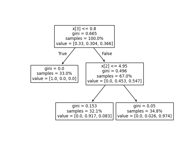
例如,在以上在虹膜資料集上建立的樹中,根節點的 value = [0.33, 0.304, 0.366],表示根節點有 33% 的類別 0 樣本、30.4% 的類別 1 樣本和 36.6% 的類別 2 樣本。我們可以將其轉換為絕對樣本數,方法是將其乘以到達根節點的樣本數,即 tree_.weighted_n_node_samples[0]。然後,根節點的 value = [37, 34, 41],表示根節點有 37 個類別 0 的樣本、34 個類別 1 的樣本和 41 個類別 2 的樣本。
遍歷樹時,樣本會分割,因此到達每個節點的 value 陣列會變更。根節點的左子節點的 value = [1., 0, 0] (或轉換為絕對樣本數時為 value = [37, 0, 0]),因為左子節點中的所有 37 個樣本都來自類別 0。
注意:在此範例中,n_outputs=1,但樹分類器也可以處理多輸出問題。每個節點的 value 陣列只會變成 2D 陣列。
我們可以將上述輸出與決策樹的圖進行比較。在此,我們顯示到達每個節點的每個類別樣本的比例,對應於 tree_.value 陣列的實際元素。
tree.plot_tree(clf, proportion=True)
plt.show()
決策路徑#
我們也可以檢索感興趣樣本的決策路徑。 decision_path 方法會輸出一個指示矩陣,讓我們能夠檢索感興趣的樣本所經過的節點。指示矩陣中位置 (i, j) 的非零元素表示樣本 i 通過節點 j。或者,對於一個樣本 i,指示矩陣中第 i 列中非零元素的位置表示該樣本所經過的節點的 ID。
可以使用 apply 方法取得感興趣樣本到達的葉節點 ID。這會返回一個陣列,其中包含每個感興趣樣本到達的葉節點 ID。使用葉節點 ID 和 decision_path,我們可以取得用於預測樣本或樣本群組的分割條件。首先,我們針對一個樣本進行操作。請注意,node_index 是一個稀疏矩陣。
node_indicator = clf.decision_path(X_test)
leaf_id = clf.apply(X_test)

sample_id = 0
# obtain ids of the nodes `sample_id` goes through, i.e., row `sample_id`
node_index = node_indicator.indices[
    node_indicator.indptr[sample_id] : node_indicator.indptr[sample_id + 1]
]

print("Rules used to predict sample {id}:\n".format(id=sample_id))
for node_id in node_index:
    # continue to the next node if it is a leaf node
    if leaf_id[sample_id] == node_id:
        continue

    # check if value of the split feature for sample 0 is below threshold
    if X_test[sample_id, feature[node_id]] <= threshold[node_id]:
        threshold_sign = "<="
    else:
        threshold_sign = ">"

    print(
        "decision node {node} : (X_test[{sample}, {feature}] = {value}) "
        "{inequality} {threshold})".format(
            node=node_id,
            sample=sample_id,
            feature=feature[node_id],
            value=X_test[sample_id, feature[node_id]],
            inequality=threshold_sign,
            threshold=threshold[node_id],
        )
    )
Rules used to predict sample 0:

decision node 0 : (X_test[0, 3] = 2.4) > 0.800000011920929)
decision node 2 : (X_test[0, 2] = 5.1) > 4.950000047683716)
對於一組樣本,我們可以確定樣本所通過的共同節點。
sample_ids = [0, 1]
# boolean array indicating the nodes both samples go through
common_nodes = node_indicator.toarray()[sample_ids].sum(axis=0) == len(sample_ids)
# obtain node ids using position in array
common_node_id = np.arange(n_nodes)[common_nodes]

print(
    "\nThe following samples {samples} share the node(s) {nodes} in the tree.".format(
        samples=sample_ids, nodes=common_node_id
    )
)
print("This is {prop}% of all nodes.".format(prop=100 * len(common_node_id) / n_nodes))
The following samples [0, 1] share the node(s) [0 2] in the tree.
This is 40.0% of all nodes.
腳本的總執行時間: (0 分鐘 0.081 秒)
相關範例