注意
前往結尾下載完整的範例程式碼。或透過 JupyterLite 或 Binder 在您的瀏覽器中執行此範例
使用 RANSAC 的穩健線性模型估計#
在此範例中,我們將了解如何使用 RANSAC 演算法穩健地將線性模型擬合到錯誤的資料。
普通的線性迴歸器對離群值敏感,而且擬合線很容易偏離資料的真實底層關係。
RANSAC 迴歸器會自動將資料分成內點和離群值,並且擬合線僅由識別出的內點決定。
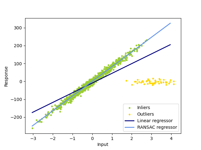
Estimated coefficients (true, linear regression, RANSAC):
82.1903908407869 [54.17236387] [82.08533159]
# Authors: The scikit-learn developers
# SPDX-License-Identifier: BSD-3-Clause

import numpy as np
from matplotlib import pyplot as plt

from sklearn import datasets, linear_model

n_samples = 1000
n_outliers = 50


X, y, coef = datasets.make_regression(
    n_samples=n_samples,
    n_features=1,
    n_informative=1,
    noise=10,
    coef=True,
    random_state=0,
)

# Add outlier data
np.random.seed(0)
X[:n_outliers] = 3 + 0.5 * np.random.normal(size=(n_outliers, 1))
y[:n_outliers] = -3 + 10 * np.random.normal(size=n_outliers)

# Fit line using all data
lr = linear_model.LinearRegression()
lr.fit(X, y)

# Robustly fit linear model with RANSAC algorithm
ransac = linear_model.RANSACRegressor()
ransac.fit(X, y)
inlier_mask = ransac.inlier_mask_
outlier_mask = np.logical_not(inlier_mask)

# Predict data of estimated models
line_X = np.arange(X.min(), X.max())[:, np.newaxis]
line_y = lr.predict(line_X)
line_y_ransac = ransac.predict(line_X)

# Compare estimated coefficients
print("Estimated coefficients (true, linear regression, RANSAC):")
print(coef, lr.coef_, ransac.estimator_.coef_)

lw = 2
plt.scatter(
    X[inlier_mask], y[inlier_mask], color="yellowgreen", marker=".", label="Inliers"
)
plt.scatter(
    X[outlier_mask], y[outlier_mask], color="gold", marker=".", label="Outliers"
)
plt.plot(line_X, line_y, color="navy", linewidth=lw, label="Linear regressor")
plt.plot(
    line_X,
    line_y_ransac,
    color="cornflowerblue",
    linewidth=lw,
    label="RANSAC regressor",
)
plt.legend(loc="lower right")
plt.xlabel("Input")
plt.ylabel("Response")
plt.show()
腳本總執行時間: (0 分鐘 0.100 秒)
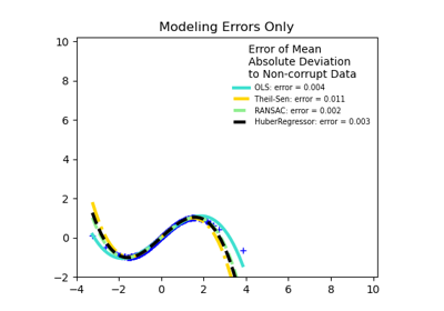
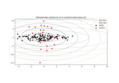
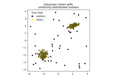
相關範例