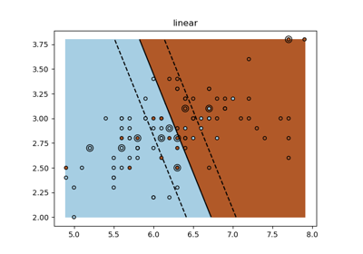
SVM 邊界範例#

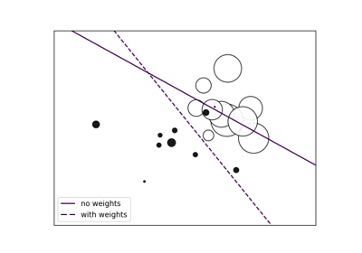
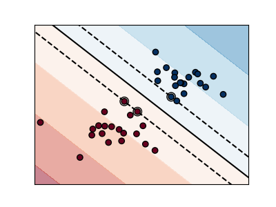
下圖說明參數 C 對分離線的影響。 C 的大值基本上告訴我們的模型，我們對資料的分佈沒有那麼大的信心，並且只會考慮接近分離線的點。

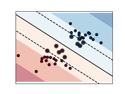
C 的小值包含更多/全部觀察值，允許使用該區域中的所有資料來計算邊界。

# Authors: The scikit-learn developers
# SPDX-License-Identifier: BSD-3-Clause

import matplotlib.pyplot as plt
import numpy as np

from sklearn import svm

# we create 40 separable points
np.random.seed(0)
X = np.r_[np.random.randn(20, 2) - [2, 2], np.random.randn(20, 2) + [2, 2]]
Y = [0] * 20 + [1] * 20

# figure number
fignum = 1

# fit the model
for name, penalty in (("unreg", 1), ("reg", 0.05)):
    clf = svm.SVC(kernel="linear", C=penalty)
    clf.fit(X, Y)

    # get the separating hyperplane
    w = clf.coef_[0]
    a = -w[0] / w[1]
    xx = np.linspace(-5, 5)
    yy = a * xx - (clf.intercept_[0]) / w[1]

    # plot the parallels to the separating hyperplane that pass through the
    # support vectors (margin away from hyperplane in direction
    # perpendicular to hyperplane). This is sqrt(1+a^2) away vertically in
    # 2-d.
    margin = 1 / np.sqrt(np.sum(clf.coef_**2))
    yy_down = yy - np.sqrt(1 + a**2) * margin
    yy_up = yy + np.sqrt(1 + a**2) * margin

    # plot the line, the points, and the nearest vectors to the plane
    plt.figure(fignum, figsize=(4, 3))
    plt.clf()
    plt.plot(xx, yy, "k-")
    plt.plot(xx, yy_down, "k--")
    plt.plot(xx, yy_up, "k--")

    plt.scatter(
        clf.support_vectors_[:, 0],
        clf.support_vectors_[:, 1],
        s=80,
        facecolors="none",
        zorder=10,
        edgecolors="k",
    )
    plt.scatter(
        X[:, 0], X[:, 1], c=Y, zorder=10, cmap=plt.get_cmap("RdBu"), edgecolors="k"
    )

    plt.axis("tight")
    x_min = -4.8
    x_max = 4.2
    y_min = -6
    y_max = 6

    YY, XX = np.meshgrid(yy, xx)
    xy = np.vstack([XX.ravel(), YY.ravel()]).T
    Z = clf.decision_function(xy).reshape(XX.shape)

    # Put the result into a contour plot
    plt.contourf(XX, YY, Z, cmap=plt.get_cmap("RdBu"), alpha=0.5, linestyles=["-"])

    plt.xlim(x_min, x_max)
    plt.ylim(y_min, y_max)

    plt.xticks(())
    plt.yticks(())
    fignum = fignum + 1

plt.show()