瑞士捲和瑞士孔降維#

此筆記本旨在比較兩種流行的非線性降維技術，T 分佈隨機鄰近嵌入 (t-SNE) 和局部線性嵌入 (LLE)，使用經典的瑞士捲資料集。然後，我們將探討它們如何處理在資料中新增一個孔洞的情況。

# Authors: The scikit-learn developers
# SPDX-License-Identifier: BSD-3-Clause

瑞士捲#

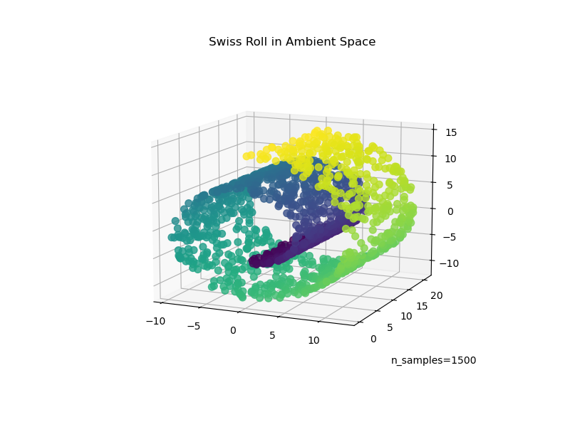
我們首先產生瑞士捲資料集。

import matplotlib.pyplot as plt

from sklearn import datasets, manifold

sr_points, sr_color = datasets.make_swiss_roll(n_samples=1500, random_state=0)

現在，讓我們看看我們的資料

fig = plt.figure(figsize=(8, 6))
ax = fig.add_subplot(111, projection="3d")
fig.add_axes(ax)
ax.scatter(
    sr_points[:, 0], sr_points[:, 1], sr_points[:, 2], c=sr_color, s=50, alpha=0.8
)
ax.set_title("Swiss Roll in Ambient Space")
ax.view_init(azim=-66, elev=12)
_ = ax.text2D(0.8, 0.05, s="n_samples=1500", transform=ax.transAxes)

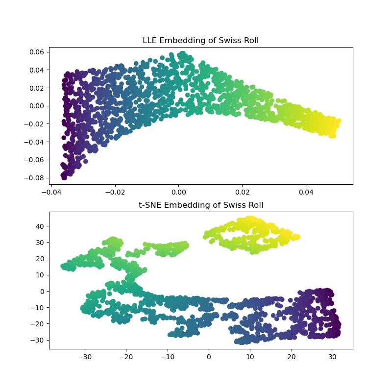
計算 LLE 和 t-SNE 嵌入，我們發現 LLE 似乎可以有效地展開瑞士捲。另一方面，t-SNE 能夠保留資料的整體結構，但對於原始資料的連續性表示效果不佳。相反，它似乎不必要地將點的區塊聚集在一起。

sr_lle, sr_err = manifold.locally_linear_embedding(
    sr_points, n_neighbors=12, n_components=2
)

sr_tsne = manifold.TSNE(n_components=2, perplexity=40, random_state=0).fit_transform(
    sr_points
)

fig, axs = plt.subplots(figsize=(8, 8), nrows=2)
axs[0].scatter(sr_lle[:, 0], sr_lle[:, 1], c=sr_color)
axs[0].set_title("LLE Embedding of Swiss Roll")
axs[1].scatter(sr_tsne[:, 0], sr_tsne[:, 1], c=sr_color)
_ = axs[1].set_title("t-SNE Embedding of Swiss Roll")

LLE Embedding of Swiss Roll, t-SNE Embedding of Swiss Roll

注意

LLE 似乎正在拉伸瑞士捲中心（紫色）的點。然而，我們觀察到這只是資料產生方式的副產品。在捲的中心附近有較高的點密度，這最終會影響 LLE 如何在較低的維度中重建資料。

瑞士孔#

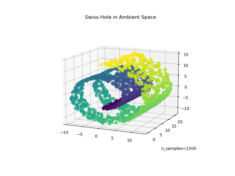
現在讓我們看看這兩種演算法如何處理在資料中新增孔洞的情況。首先，我們產生瑞士孔資料集並繪製它

sh_points, sh_color = datasets.make_swiss_roll(
    n_samples=1500, hole=True, random_state=0
)

fig = plt.figure(figsize=(8, 6))
ax = fig.add_subplot(111, projection="3d")
fig.add_axes(ax)
ax.scatter(
    sh_points[:, 0], sh_points[:, 1], sh_points[:, 2], c=sh_color, s=50, alpha=0.8
)
ax.set_title("Swiss-Hole in Ambient Space")
ax.view_init(azim=-66, elev=12)
_ = ax.text2D(0.8, 0.05, s="n_samples=1500", transform=ax.transAxes)

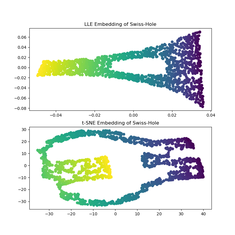
計算 LLE 和 t-SNE 嵌入，我們得到與瑞士捲相似的結果。 LLE 非常有能力展開資料，甚至保留了孔洞。 t-SNE 再次似乎將點的區塊聚集在一起，但是，我們注意到它保留了原始資料的總體拓撲結構。

sh_lle, sh_err = manifold.locally_linear_embedding(
    sh_points, n_neighbors=12, n_components=2
)

sh_tsne = manifold.TSNE(
    n_components=2, perplexity=40, init="random", random_state=0
).fit_transform(sh_points)

fig, axs = plt.subplots(figsize=(8, 8), nrows=2)
axs[0].scatter(sh_lle[:, 0], sh_lle[:, 1], c=sh_color)
axs[0].set_title("LLE Embedding of Swiss-Hole")
axs[1].scatter(sh_tsne[:, 0], sh_tsne[:, 1], c=sh_color)
_ = axs[1].set_title("t-SNE Embedding of Swiss-Hole")