特徵縮放的重要性#

透過標準化進行特徵縮放，也稱為 Z 分數正規化，是許多機器學習演算法的重要預處理步驟。它涉及重新縮放每個特徵，使其標準差為 1，平均值為 0。

即使基於樹的模型（幾乎）不受縮放的影響，許多其他演算法仍需要正規化特徵，通常出於不同的原因：為了簡化收斂（例如非懲罰邏輯回歸），以建立與未縮放資料的擬合完全不同的模型擬合（例如 KNeighbors 模型）。後者在本範例的第一部分中示範。

在本範例的第二部分中，我們展示了主成分分析 (PCA) 如何受到特徵正規化的影響。為了說明這一點，我們比較了使用PCA在未縮放資料上找到的主成分與首先使用StandardScaler縮放資料時獲得的主成分。

在本範例的最後一部分中，我們展示了正規化對在 PCA 縮減資料上訓練的模型準確性的影響。

# Authors: The scikit-learn developers
# SPDX-License-Identifier: BSD-3-Clause

載入並準備資料#

使用的資料集是 UCI 提供的葡萄酒識別資料集。此資料集具有連續特徵，這些特徵由於測量的不同屬性（例如酒精含量和蘋果酸）而在規模上是異質的。

from sklearn.datasets import load_wine
from sklearn.model_selection import train_test_split
from sklearn.preprocessing import StandardScaler

X, y = load_wine(return_X_y=True, as_frame=True)
scaler = StandardScaler().set_output(transform="pandas")

X_train, X_test, y_train, y_test = train_test_split(
    X, y, test_size=0.30, random_state=42
)
scaled_X_train = scaler.fit_transform(X_train)

重新縮放對 k 近鄰模型的影響#

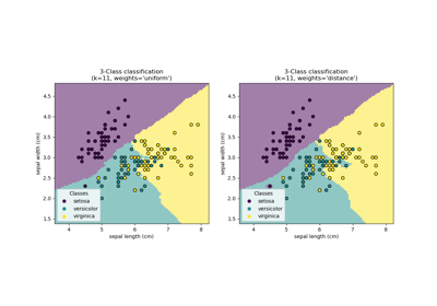
為了視覺化KNeighborsClassifier的決策邊界，在本節中，我們選擇一個具有不同數量級值的 2 個特徵的子集。

請記住，使用特徵的子集來訓練模型很可能會遺漏具有高預測影響的特徵，導致決策邊界比在完整特徵集上訓練的模型差得多。

import matplotlib.pyplot as plt

from sklearn.inspection import DecisionBoundaryDisplay
from sklearn.neighbors import KNeighborsClassifier

X_plot = X[["proline", "hue"]]
X_plot_scaled = scaler.fit_transform(X_plot)
clf = KNeighborsClassifier(n_neighbors=20)


def fit_and_plot_model(X_plot, y, clf, ax):
    clf.fit(X_plot, y)
    disp = DecisionBoundaryDisplay.from_estimator(
        clf,
        X_plot,
        response_method="predict",
        alpha=0.5,
        ax=ax,
    )
    disp.ax_.scatter(X_plot["proline"], X_plot["hue"], c=y, s=20, edgecolor="k")
    disp.ax_.set_xlim((X_plot["proline"].min(), X_plot["proline"].max()))
    disp.ax_.set_ylim((X_plot["hue"].min(), X_plot["hue"].max()))
    return disp.ax_


fig, (ax1, ax2) = plt.subplots(ncols=2, figsize=(12, 6))

fit_and_plot_model(X_plot, y, clf, ax1)
ax1.set_title("KNN without scaling")

fit_and_plot_model(X_plot_scaled, y, clf, ax2)
ax2.set_xlabel("scaled proline")
ax2.set_ylabel("scaled hue")
_ = ax2.set_title("KNN with scaling")

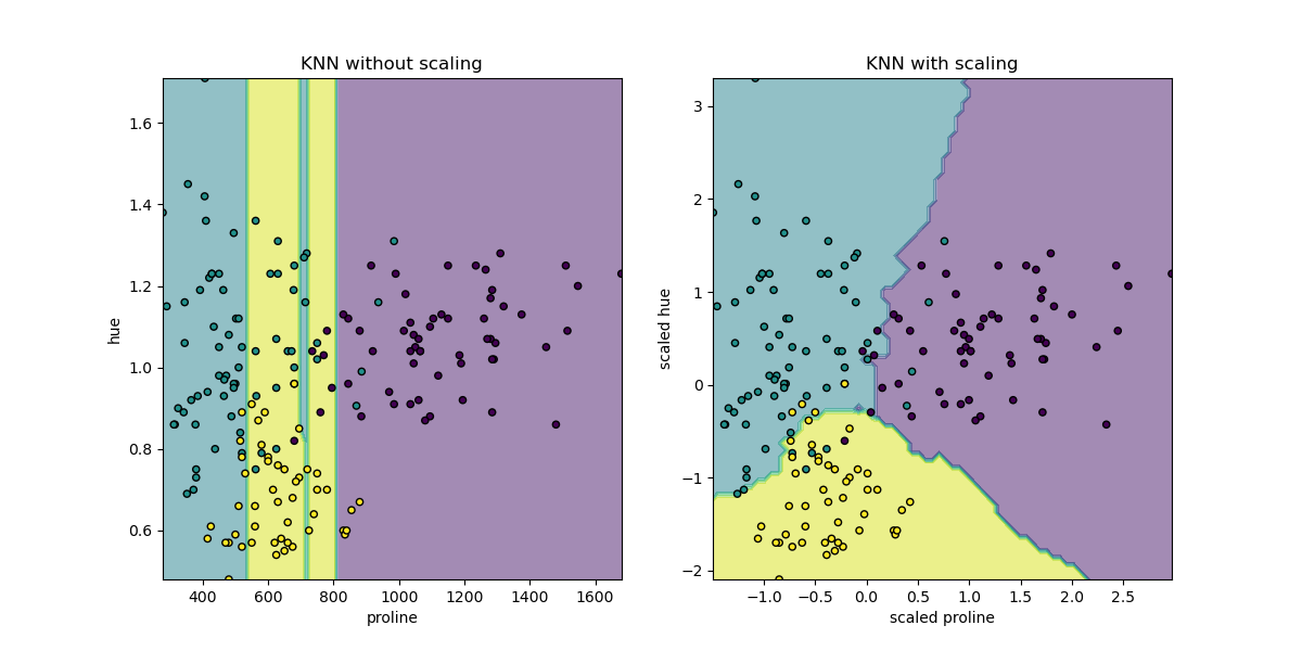
此處的決策邊界顯示，擬合縮放或未縮放的資料會導致完全不同的模型。原因是變數「proline」的值在 0 到 1,000 之間變化；而變數「hue」在 1 到 10 之間變化。因此，樣本之間的距離主要受到「proline」值差異的影響，而「hue」的值將被相對忽略。如果使用StandardScaler來正規化此資料庫，則兩個縮放值都大約在 -3 到 3 之間，並且鄰近結構將或多或少受到兩個變數的同等影響。

重新縮放對 PCA 降維的影響#

使用PCA進行降維包括找到最大化變異數的特徵。如果一個特徵僅僅由於其各自的縮放而比其他特徵變化更大，則PCA將確定該特徵主導主成分的方向。

我們可以檢查使用所有原始特徵的第一個主成分

import pandas as pd

from sklearn.decomposition import PCA

pca = PCA(n_components=2).fit(X_train)
scaled_pca = PCA(n_components=2).fit(scaled_X_train)
X_train_transformed = pca.transform(X_train)
X_train_std_transformed = scaled_pca.transform(scaled_X_train)

first_pca_component = pd.DataFrame(
    pca.components_[0], index=X.columns, columns=["without scaling"]
)
first_pca_component["with scaling"] = scaled_pca.components_[0]
first_pca_component.plot.bar(
    title="Weights of the first principal component", figsize=(6, 8)
)

_ = plt.tight_layout()

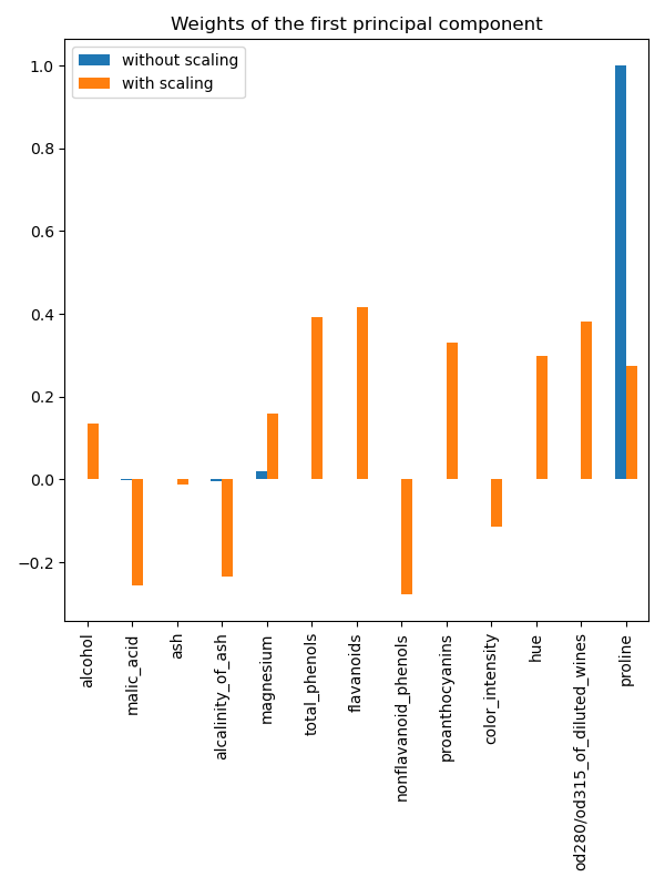
Weights of the first principal component

事實上，我們發現「proline」特徵在沒有縮放的情況下主導了第一個主成分的方向，比其他特徵高出約兩個數量級。當觀察縮放版本的資料的第一個主成分時，情況會有所不同，其中所有特徵的數量級大致相同。

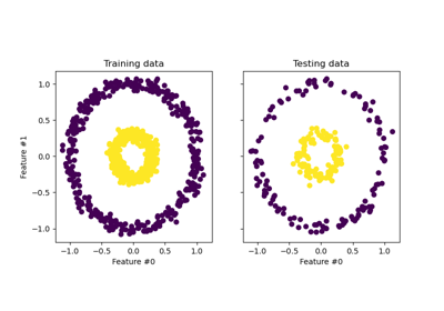
我們可以視覺化兩種情況下主成分的分佈

fig, (ax1, ax2) = plt.subplots(nrows=1, ncols=2, figsize=(10, 5))

target_classes = range(0, 3)
colors = ("blue", "red", "green")
markers = ("^", "s", "o")

for target_class, color, marker in zip(target_classes, colors, markers):
    ax1.scatter(
        x=X_train_transformed[y_train == target_class, 0],
        y=X_train_transformed[y_train == target_class, 1],
        color=color,
        label=f"class {target_class}",
        alpha=0.5,
        marker=marker,
    )

    ax2.scatter(
        x=X_train_std_transformed[y_train == target_class, 0],
        y=X_train_std_transformed[y_train == target_class, 1],
        color=color,
        label=f"class {target_class}",
        alpha=0.5,
        marker=marker,
    )

ax1.set_title("Unscaled training dataset after PCA")
ax2.set_title("Standardized training dataset after PCA")

for ax in (ax1, ax2):
    ax.set_xlabel("1st principal component")
    ax.set_ylabel("2nd principal component")
    ax.legend(loc="upper right")
    ax.grid()

_ = plt.tight_layout()

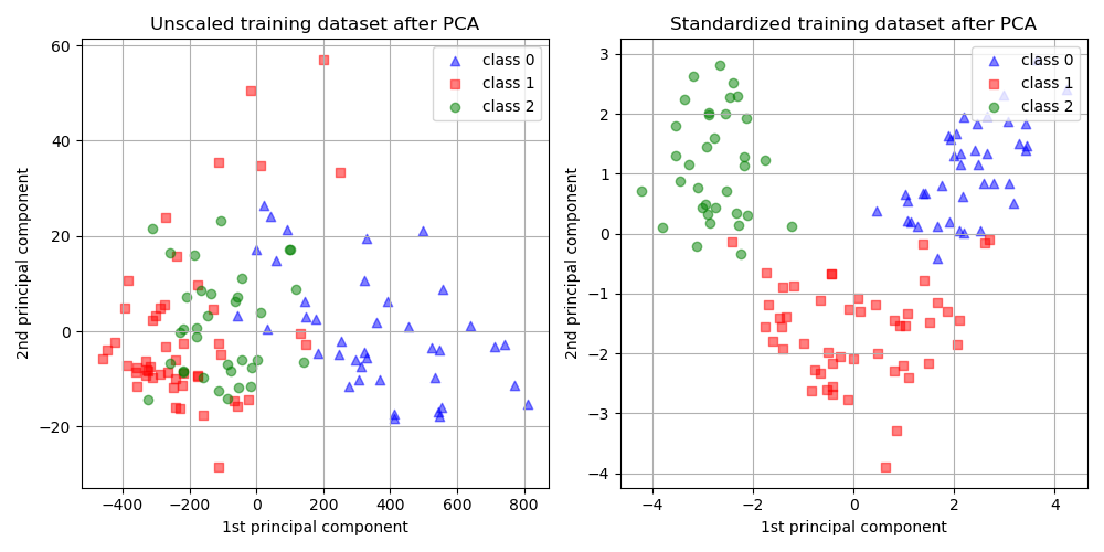
Unscaled training dataset after PCA, Standardized training dataset after PCA

從上面的圖中，我們觀察到在降低維度之前縮放特徵會產生數量級相同的成分。在這種情況下，它還提高了類別的可分離性。事實上，在下一節中，我們確認更好的可分離性對整體模型效能有良好的影響。

重新縮放對模型效能的影響#

首先，我們展示了LogisticRegressionCV的最佳正規化如何取決於資料的縮放或非縮放

import numpy as np

from sklearn.linear_model import LogisticRegressionCV
from sklearn.pipeline import make_pipeline

Cs = np.logspace(-5, 5, 20)

unscaled_clf = make_pipeline(pca, LogisticRegressionCV(Cs=Cs))
unscaled_clf.fit(X_train, y_train)

scaled_clf = make_pipeline(scaler, pca, LogisticRegressionCV(Cs=Cs))
scaled_clf.fit(X_train, y_train)

print(f"Optimal C for the unscaled PCA: {unscaled_clf[-1].C_[0]:.4f}\n")
print(f"Optimal C for the standardized data with PCA: {scaled_clf[-1].C_[0]:.2f}")

Optimal C for the unscaled PCA: 0.0004

Optimal C for the standardized data with PCA: 20.69

對於在套用 PCA 之前未縮放的資料，正規化的需求較高（C的值較低）。我們現在評估縮放對最佳模型的準確性和平均對數損失的影響

from sklearn.metrics import accuracy_score, log_loss

y_pred = unscaled_clf.predict(X_test)
y_pred_scaled = scaled_clf.predict(X_test)
y_proba = unscaled_clf.predict_proba(X_test)
y_proba_scaled = scaled_clf.predict_proba(X_test)

print("Test accuracy for the unscaled PCA")
print(f"{accuracy_score(y_test, y_pred):.2%}\n")
print("Test accuracy for the standardized data with PCA")
print(f"{accuracy_score(y_test, y_pred_scaled):.2%}\n")
print("Log-loss for the unscaled PCA")
print(f"{log_loss(y_test, y_proba):.3}\n")
print("Log-loss for the standardized data with PCA")
print(f"{log_loss(y_test, y_proba_scaled):.3}")

Test accuracy for the unscaled PCA
35.19%

Test accuracy for the standardized data with PCA
96.30%

Log-loss for the unscaled PCA
0.957

Log-loss for the standardized data with PCA
0.0825

當資料在PCA之前縮放時，觀察到預測準確性存在明顯差異，因為它大大優於未縮放版本。這與從上一節的圖中獲得的直觀概念一致，其中當在使用PCA之前縮放時，組件會變成線性可分離的。

請注意，在這種情況下，具有縮放特徵的模型比具有未縮放特徵的模型表現更好，因為預期所有變數都具有預測性，而且我們寧願避免其中一些變數被相對忽略。

如果較小規模的變數不具有預測性，則在縮放特徵後可能會導致效能下降：雜訊特徵在縮放後將對預測做出更多貢獻，因此縮放將增加過度擬合。

最後但並非最不重要的一點是，我們觀察到透過縮放步驟可以獲得較低的對數損失。

腳本總執行時間： (0 分鐘 1.966 秒)