F 檢定和互資訊的比較#

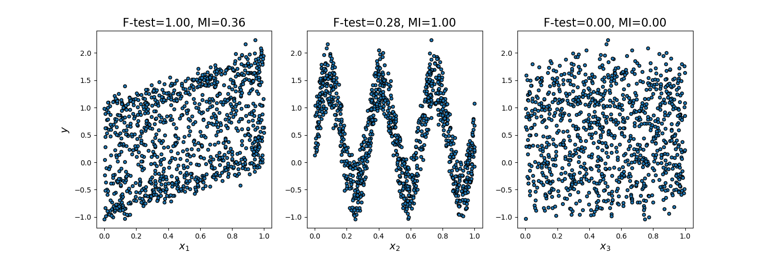
此範例說明單變量 F 檢定統計量和互資訊之間的差異。

我們考慮 3 個特徵 x_1、x_2、x_3 在 [0, 1] 上均勻分佈，目標依賴於它們，如下所示

y = x_1 + sin(6 * pi * x_2) + 0.1 * N(0, 1)，也就是說第三個特徵完全不相關。

下面的程式碼繪製了 y 對個別 x_i 的依賴關係，以及單變量 F 檢定統計量和互資訊的標準化值。

由於 F 檢定僅捕獲線性依賴關係，因此它將 x_1 評為最具區別性的特徵。另一方面，互資訊可以捕獲變數之間的任何依賴關係，並且它將 x_2 評為最具區別性的特徵，這可能更符合我們對此範例的直觀感受。兩種方法都正確地將 x_3 標記為不相關。

F-test=1.00, MI=0.36, F-test=0.28, MI=1.00, F-test=0.00, MI=0.00

# Authors: The scikit-learn developers
# SPDX-License-Identifier: BSD-3-Clause

import matplotlib.pyplot as plt
import numpy as np

from sklearn.feature_selection import f_regression, mutual_info_regression

np.random.seed(0)
X = np.random.rand(1000, 3)
y = X[:, 0] + np.sin(6 * np.pi * X[:, 1]) + 0.1 * np.random.randn(1000)

f_test, _ = f_regression(X, y)
f_test /= np.max(f_test)

mi = mutual_info_regression(X, y)
mi /= np.max(mi)

plt.figure(figsize=(15, 5))
for i in range(3):
    plt.subplot(1, 3, i + 1)
    plt.scatter(X[:, i], y, edgecolor="black", s=20)
    plt.xlabel("$x_{}$".format(i + 1), fontsize=14)
    if i == 0:
        plt.ylabel("$y$", fontsize=14)
    plt.title("F-test={:.2f}, MI={:.2f}".format(f_test[i], mi[i]), fontsize=16)
plt.show()