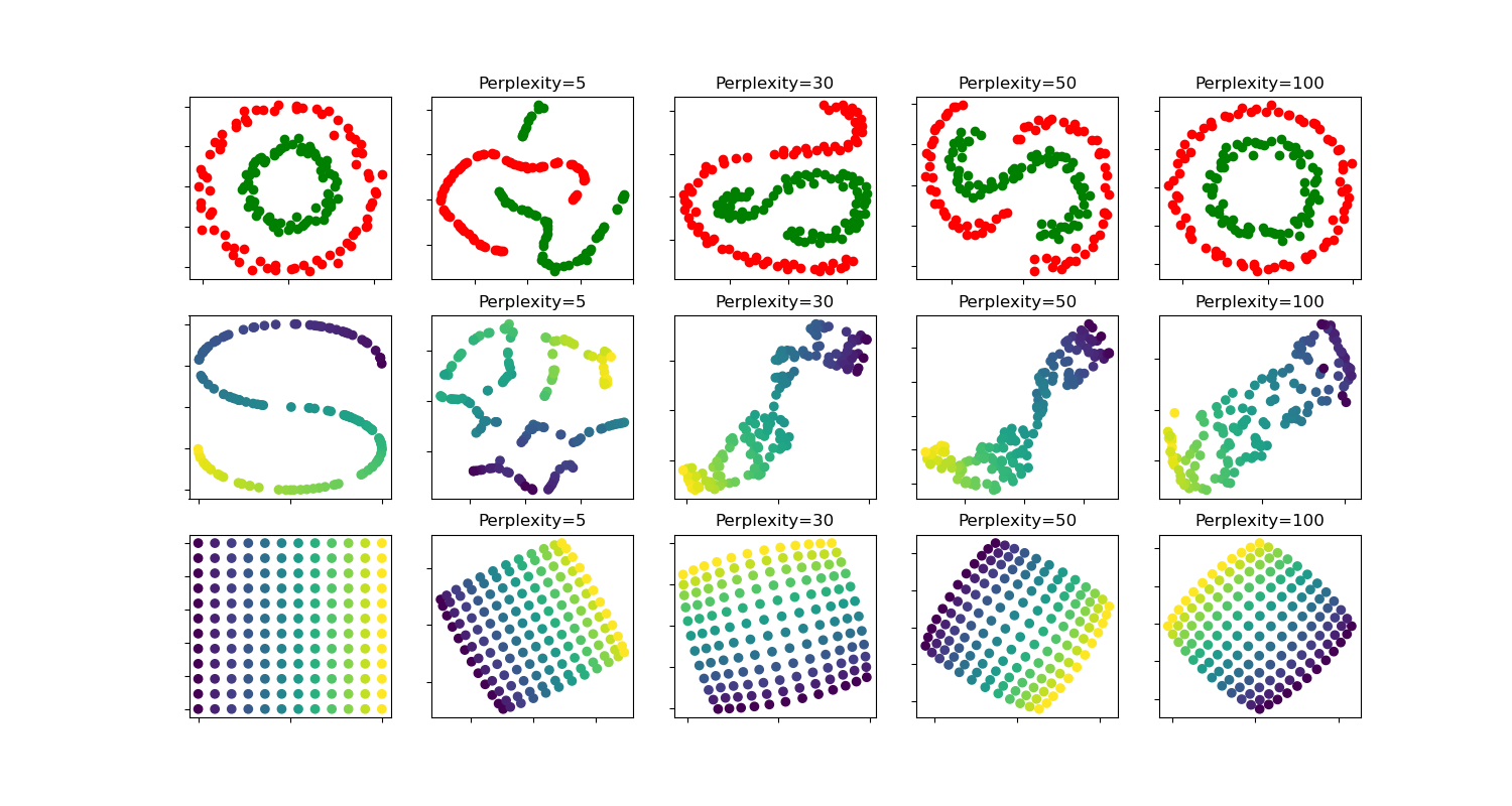
t-SNE：各種困惑值對形狀的影響#

t-SNE 在兩個同心圓和 S 曲線數據集上針對不同困惑值的說明。

我們觀察到，隨著困惑值的增加，形狀趨於更清晰。

叢集的大小、距離和形狀可能會因初始化、困惑值而異，而且並不總是傳達意義。

如下所示，對於較高的困惑度，t-SNE 找到了兩個同心圓的有意義拓撲結構，但是圓的大小和距離與原始略有不同。與兩個圓的數據集相反，即使對於較大的困惑度值，S 曲線數據集上的形狀在視覺上也偏離了 S 曲線拓撲結構。

有關更多詳細資訊，「如何有效地使用 t-SNE」 https://distill.pub/2016/misread-tsne/ 提供了對各種參數影響的良好討論，以及探索這些影響的互動式圖表。

Perplexity=5, Perplexity=30, Perplexity=50, Perplexity=100, Perplexity=5, Perplexity=30, Perplexity=50, Perplexity=100, Perplexity=5, Perplexity=30, Perplexity=50, Perplexity=100

circles, perplexity=5 in 0.17 sec
circles, perplexity=30 in 0.28 sec
circles, perplexity=50 in 0.23 sec
circles, perplexity=100 in 0.26 sec
S-curve, perplexity=5 in 0.13 sec
S-curve, perplexity=30 in 0.2 sec
S-curve, perplexity=50 in 0.24 sec
S-curve, perplexity=100 in 0.23 sec
uniform grid, perplexity=5 in 0.2 sec
uniform grid, perplexity=30 in 0.27 sec
uniform grid, perplexity=50 in 0.27 sec
uniform grid, perplexity=100 in 0.27 sec

# Authors: The scikit-learn developers
# SPDX-License-Identifier: BSD-3-Clause

from time import time

import matplotlib.pyplot as plt
import numpy as np
from matplotlib.ticker import NullFormatter

from sklearn import datasets, manifold

n_samples = 150
n_components = 2
(fig, subplots) = plt.subplots(3, 5, figsize=(15, 8))
perplexities = [5, 30, 50, 100]

X, y = datasets.make_circles(
    n_samples=n_samples, factor=0.5, noise=0.05, random_state=0
)

red = y == 0
green = y == 1

ax = subplots[0][0]
ax.scatter(X[red, 0], X[red, 1], c="r")
ax.scatter(X[green, 0], X[green, 1], c="g")
ax.xaxis.set_major_formatter(NullFormatter())
ax.yaxis.set_major_formatter(NullFormatter())
plt.axis("tight")

for i, perplexity in enumerate(perplexities):
    ax = subplots[0][i + 1]

    t0 = time()
    tsne = manifold.TSNE(
        n_components=n_components,
        init="random",
        random_state=0,
        perplexity=perplexity,
        max_iter=300,
    )
    Y = tsne.fit_transform(X)
    t1 = time()
    print("circles, perplexity=%d in %.2g sec" % (perplexity, t1 - t0))
    ax.set_title("Perplexity=%d" % perplexity)
    ax.scatter(Y[red, 0], Y[red, 1], c="r")
    ax.scatter(Y[green, 0], Y[green, 1], c="g")
    ax.xaxis.set_major_formatter(NullFormatter())
    ax.yaxis.set_major_formatter(NullFormatter())
    ax.axis("tight")

# Another example using s-curve
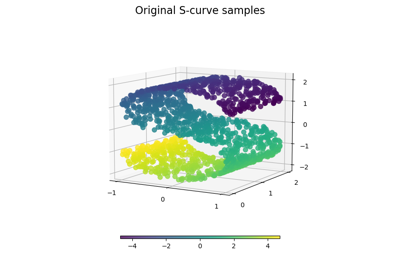
X, color = datasets.make_s_curve(n_samples, random_state=0)

ax = subplots[1][0]
ax.scatter(X[:, 0], X[:, 2], c=color)
ax.xaxis.set_major_formatter(NullFormatter())
ax.yaxis.set_major_formatter(NullFormatter())

for i, perplexity in enumerate(perplexities):
    ax = subplots[1][i + 1]

    t0 = time()
    tsne = manifold.TSNE(
        n_components=n_components,
        init="random",
        random_state=0,
        perplexity=perplexity,
        learning_rate="auto",
        max_iter=300,
    )
    Y = tsne.fit_transform(X)
    t1 = time()
    print("S-curve, perplexity=%d in %.2g sec" % (perplexity, t1 - t0))

    ax.set_title("Perplexity=%d" % perplexity)
    ax.scatter(Y[:, 0], Y[:, 1], c=color)
    ax.xaxis.set_major_formatter(NullFormatter())
    ax.yaxis.set_major_formatter(NullFormatter())
    ax.axis("tight")


# Another example using a 2D uniform grid
x = np.linspace(0, 1, int(np.sqrt(n_samples)))
xx, yy = np.meshgrid(x, x)
X = np.hstack(
    [
        xx.ravel().reshape(-1, 1),
        yy.ravel().reshape(-1, 1),
    ]
)
color = xx.ravel()
ax = subplots[2][0]
ax.scatter(X[:, 0], X[:, 1], c=color)
ax.xaxis.set_major_formatter(NullFormatter())
ax.yaxis.set_major_formatter(NullFormatter())

for i, perplexity in enumerate(perplexities):
    ax = subplots[2][i + 1]

    t0 = time()
    tsne = manifold.TSNE(
        n_components=n_components,
        init="random",
        random_state=0,
        perplexity=perplexity,
        max_iter=400,
    )
    Y = tsne.fit_transform(X)
    t1 = time()
    print("uniform grid, perplexity=%d in %.2g sec" % (perplexity, t1 - t0))

    ax.set_title("Perplexity=%d" % perplexity)
    ax.scatter(Y[:, 0], Y[:, 1], c=color)
    ax.xaxis.set_major_formatter(NullFormatter())
    ax.yaxis.set_major_formatter(NullFormatter())
    ax.axis("tight")


plt.show()