Theil-Sen 迴歸#

在合成資料集上計算 Theil-Sen 迴歸。

有關迴歸器的更多資訊，請參閱 Theil-Sen 估計器：基於廣義中位數的估計器。

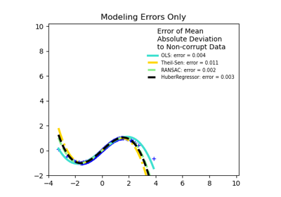
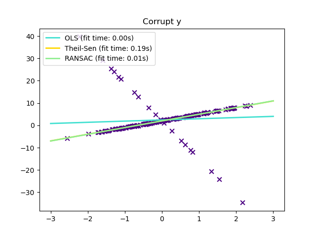
與 OLS（普通最小平方法）估計器相比，Theil-Sen 估計器對離群值具有穩健性。在簡單線性迴歸的情況下，它的崩潰點約為 29.3%，這意味著它可以容忍高達 29.3% 的任意損壞資料（離群值）在二維情況下。

模型的估計是透過計算 p 個子樣本點所有可能組合的子族群的斜率和截距來完成的。如果擬合截距，則 p 必須大於或等於 n_features + 1。最終的斜率和截距然後定義為這些斜率和截距的空間中位數。

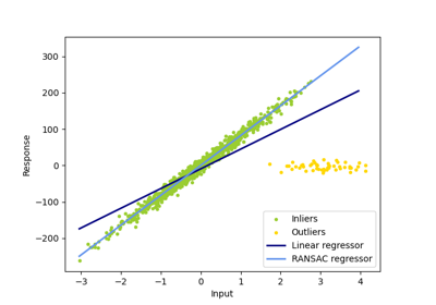
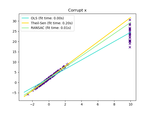
在某些情況下，Theil-Sen 的表現優於 RANSAC，RANSAC 也是一種穩健的方法。這在下面的第二個範例中說明，其中關於 x 軸的離群值會擾亂 RANSAC。調整 RANSAC 的 residual_threshold 參數可以補救這種情況，但通常需要關於資料和離群值性質的先驗知識。由於 Theil-Sen 的計算複雜性，建議僅將其用於樣本和特徵數量方面的小問題。對於較大的問題，max_subpopulation 參數將 p 個子樣本點的所有可能組合的大小限制為隨機選擇的子集，因此也限制了執行時間。因此，Theil-Sen 適用於較大的問題，但缺點是會失去其某些數學屬性，因為它是在隨機子集上運作。

# Authors: The scikit-learn developers
# SPDX-License-Identifier: BSD-3-Clause

import time

import matplotlib.pyplot as plt
import numpy as np

from sklearn.linear_model import LinearRegression, RANSACRegressor, TheilSenRegressor

estimators = [
    ("OLS", LinearRegression()),
    ("Theil-Sen", TheilSenRegressor(random_state=42)),
    ("RANSAC", RANSACRegressor(random_state=42)),
]
colors = {"OLS": "turquoise", "Theil-Sen": "gold", "RANSAC": "lightgreen"}
lw = 2

僅在 y 方向的離群值#

np.random.seed(0)
n_samples = 200
# Linear model y = 3*x + N(2, 0.1**2)
x = np.random.randn(n_samples)
w = 3.0
c = 2.0
noise = 0.1 * np.random.randn(n_samples)
y = w * x + c + noise
# 10% outliers
y[-20:] += -20 * x[-20:]
X = x[:, np.newaxis]

plt.scatter(x, y, color="indigo", marker="x", s=40)
line_x = np.array([-3, 3])
for name, estimator in estimators:
    t0 = time.time()
    estimator.fit(X, y)
    elapsed_time = time.time() - t0
    y_pred = estimator.predict(line_x.reshape(2, 1))
    plt.plot(
        line_x,
        y_pred,
        color=colors[name],
        linewidth=lw,
        label="%s (fit time: %.2fs)" % (name, elapsed_time),
    )

plt.axis("tight")
plt.legend(loc="upper left")
_ = plt.title("Corrupt y")

在 X 方向的離群值#

np.random.seed(0)
# Linear model y = 3*x + N(2, 0.1**2)
x = np.random.randn(n_samples)
noise = 0.1 * np.random.randn(n_samples)
y = 3 * x + 2 + noise
# 10% outliers
x[-20:] = 9.9
y[-20:] += 22
X = x[:, np.newaxis]

plt.figure()
plt.scatter(x, y, color="indigo", marker="x", s=40)

line_x = np.array([-3, 10])
for name, estimator in estimators:
    t0 = time.time()
    estimator.fit(X, y)
    elapsed_time = time.time() - t0
    y_pred = estimator.predict(line_x.reshape(2, 1))
    plt.plot(
        line_x,
        y_pred,
        color=colors[name],
        linewidth=lw,
        label="%s (fit time: %.2fs)" % (name, elapsed_time),
    )

plt.axis("tight")
plt.legend(loc="upper left")
plt.title("Corrupt x")
plt.show()