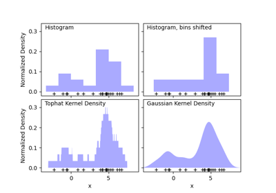
核密度估計#

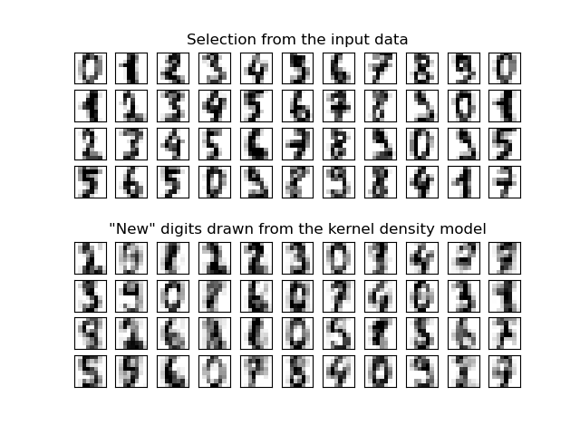
此範例說明如何使用核密度估計 (KDE)，這是一種強大的非參數密度估計技術，來學習數據集的生成模型。有了這個生成模型，就可以繪製新的樣本。這些新樣本反映了數據的基礎模型。

best bandwidth: 3.79269019073225

# Authors: The scikit-learn developers
# SPDX-License-Identifier: BSD-3-Clause

import matplotlib.pyplot as plt
import numpy as np

from sklearn.datasets import load_digits
from sklearn.decomposition import PCA
from sklearn.model_selection import GridSearchCV
from sklearn.neighbors import KernelDensity

# load the data
digits = load_digits()

# project the 64-dimensional data to a lower dimension
pca = PCA(n_components=15, whiten=False)
data = pca.fit_transform(digits.data)

# use grid search cross-validation to optimize the bandwidth
params = {"bandwidth": np.logspace(-1, 1, 20)}
grid = GridSearchCV(KernelDensity(), params)
grid.fit(data)

print("best bandwidth: {0}".format(grid.best_estimator_.bandwidth))

# use the best estimator to compute the kernel density estimate
kde = grid.best_estimator_

# sample 44 new points from the data
new_data = kde.sample(44, random_state=0)
new_data = pca.inverse_transform(new_data)

# turn data into a 4x11 grid
new_data = new_data.reshape((4, 11, -1))
real_data = digits.data[:44].reshape((4, 11, -1))

# plot real digits and resampled digits
fig, ax = plt.subplots(9, 11, subplot_kw=dict(xticks=[], yticks=[]))
for j in range(11):
    ax[4, j].set_visible(False)
    for i in range(4):
        im = ax[i, j].imshow(
            real_data[i, j].reshape((8, 8)), cmap=plt.cm.binary, interpolation="nearest"
        )
        im.set_clim(0, 16)
        im = ax[i + 5, j].imshow(
            new_data[i, j].reshape((8, 8)), cmap=plt.cm.binary, interpolation="nearest"
        )
        im.set_clim(0, 16)

ax[0, 5].set_title("Selection from the input data")
ax[5, 5].set_title('"New" digits drawn from the kernel density model')

plt.show()