真實資料集上的離群值偵測#

此範例說明在真實資料集中需要穩健的共變異數估計。這對於離群值偵測和更好地理解資料結構都很有用。

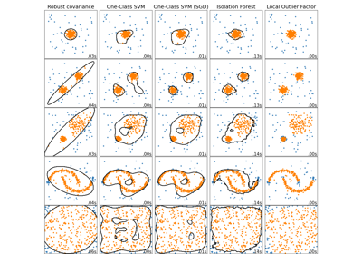
我們從葡萄酒資料集中選擇了兩組兩個變數，以說明可以使用幾種離群值偵測工具進行哪種分析。為了視覺化，我們使用二維範例，但應該意識到在高維度中情況並非如此簡單，正如將要指出的那樣。

在下面的兩個範例中，主要結果是非穩健的經驗共變異數估計會受到觀察值異質結構的很大影響。儘管穩健的共變異數估計能夠集中在資料分佈的主要模式上，但它仍然堅持認為資料應該是高斯分佈的假設，從而對資料結構產生一些有偏差的估計，但在某種程度上仍然準確。單類別 SVM 不假設資料分佈的任何參數形式，因此可以更好地對資料的複雜形狀進行建模。

# Authors: The scikit-learn developers
# SPDX-License-Identifier: BSD-3-Clause

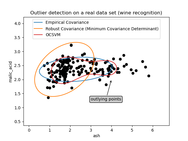
第一個範例#

第一個範例說明，當存在離群點時，最小共變異數行列式穩健估計器如何幫助集中在相關的群集上。此處，經驗共變異數估計會因主要群集外的點而扭曲。當然，一些篩選工具會指出存在兩個群集（支援向量機、高斯混合模型、單變數離群值偵測，...）。但是，如果它是高維度範例，則這些都無法如此輕鬆地應用。

from sklearn.covariance import EllipticEnvelope
from sklearn.inspection import DecisionBoundaryDisplay
from sklearn.svm import OneClassSVM

estimators = {
    "Empirical Covariance": EllipticEnvelope(support_fraction=1.0, contamination=0.25),
    "Robust Covariance (Minimum Covariance Determinant)": EllipticEnvelope(
        contamination=0.25
    ),
    "OCSVM": OneClassSVM(nu=0.25, gamma=0.35),
}

import matplotlib.lines as mlines
import matplotlib.pyplot as plt

from sklearn.datasets import load_wine

X = load_wine()["data"][:, [1, 2]]  # two clusters

fig, ax = plt.subplots()
colors = ["tab:blue", "tab:orange", "tab:red"]
# Learn a frontier for outlier detection with several classifiers
legend_lines = []
for color, (name, estimator) in zip(colors, estimators.items()):
    estimator.fit(X)
    DecisionBoundaryDisplay.from_estimator(
        estimator,
        X,
        response_method="decision_function",
        plot_method="contour",
        levels=[0],
        colors=color,
        ax=ax,
    )
    legend_lines.append(mlines.Line2D([], [], color=color, label=name))


ax.scatter(X[:, 0], X[:, 1], color="black")
bbox_args = dict(boxstyle="round", fc="0.8")
arrow_args = dict(arrowstyle="->")
ax.annotate(
    "outlying points",
    xy=(4, 2),
    xycoords="data",
    textcoords="data",
    xytext=(3, 1.25),
    bbox=bbox_args,
    arrowprops=arrow_args,
)
ax.legend(handles=legend_lines, loc="upper center")
_ = ax.set(
    xlabel="ash",
    ylabel="malic_acid",
    title="Outlier detection on a real data set (wine recognition)",
)

Outlier detection on a real data set (wine recognition)

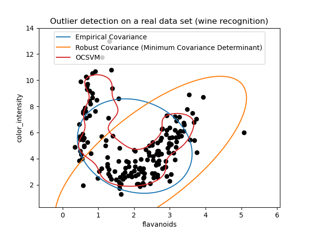
第二個範例#

第二個範例顯示了最小共變異數行列式穩健共變異數估計器能夠集中在資料分佈的主要模式上的能力：儘管由於香蕉形分佈而難以估計共變異數，但位置似乎被很好地估計了。無論如何，我們可以擺脫一些離群的觀察值。單類別 SVM 能夠捕捉真實的資料結構，但困難之處在於調整其核心頻寬參數，以便在資料散佈矩陣的形狀和過擬合資料的風險之間取得良好的折衷。

X = load_wine()["data"][:, [6, 9]]  # "banana"-shaped

fig, ax = plt.subplots()
colors = ["tab:blue", "tab:orange", "tab:red"]
# Learn a frontier for outlier detection with several classifiers
legend_lines = []
for color, (name, estimator) in zip(colors, estimators.items()):
    estimator.fit(X)
    DecisionBoundaryDisplay.from_estimator(
        estimator,
        X,
        response_method="decision_function",
        plot_method="contour",
        levels=[0],
        colors=color,
        ax=ax,
    )
    legend_lines.append(mlines.Line2D([], [], color=color, label=name))


ax.scatter(X[:, 0], X[:, 1], color="black")
ax.legend(handles=legend_lines, loc="upper center")
ax.set(
    xlabel="flavanoids",
    ylabel="color_intensity",
    title="Outlier detection on a real data set (wine recognition)",
)

plt.show()