scikit-learn 0.24 的版本重點

我們很高興宣佈發佈 scikit-learn 0.24！添加了許多錯誤修復和改進，以及一些新的主要功能。我們在下面詳細介紹此版本的一些主要功能。如需所有變更的詳盡清單，請參閱版本說明。

若要安裝最新版本 (使用 pip)

pip install --upgrade scikit-learn

或使用 conda

conda install -c conda-forge scikit-learn

用於調整超參數的連續減半估計器

連續減半是一種先進的方法，現在可用於探索參數空間並識別其最佳組合。HalvingGridSearchCV 和 HalvingRandomSearchCV 可以用作 GridSearchCV 和 RandomizedSearchCV 的直接替代品。連續減半是一個迭代選擇過程，如下圖所示。第一次迭代使用少量資源執行，其中資源通常對應於訓練樣本的數量，但也可以是任意整數參數，例如隨機森林中的 n_estimators。僅選擇參數候選的子集進行下一次迭代，該迭代將使用增加的資源量來執行。只有候選的子集會持續到迭代過程結束，而最佳參數候選是上次迭代中得分最高的那個。

請在使用者指南中閱讀更多內容（注意：連續減半估計器仍然是實驗性的）。

import numpy as np
from scipy.stats import randint
from sklearn.experimental import enable_halving_search_cv  # noqa
from sklearn.model_selection import HalvingRandomSearchCV
from sklearn.ensemble import RandomForestClassifier
from sklearn.datasets import make_classification

rng = np.random.RandomState(0)

X, y = make_classification(n_samples=700, random_state=rng)

clf = RandomForestClassifier(n_estimators=10, random_state=rng)

param_dist = {
    "max_depth": [3, None],
    "max_features": randint(1, 11),
    "min_samples_split": randint(2, 11),
    "bootstrap": [True, False],
    "criterion": ["gini", "entropy"],
}

rsh = HalvingRandomSearchCV(
    estimator=clf, param_distributions=param_dist, factor=2, random_state=rng
)
rsh.fit(X, y)
rsh.best_params_

{'bootstrap': True, 'criterion': 'gini', 'max_depth': None, 'max_features': 10, 'min_samples_split': 10}

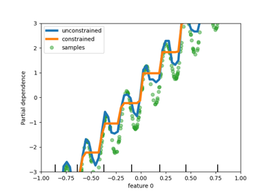
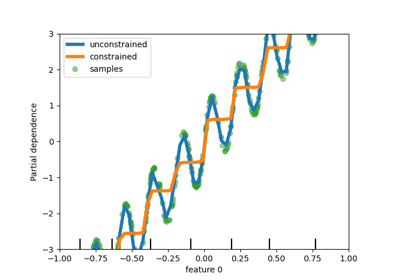
HistGradientBoosting 估計器中對類別特徵的本機支援

HistGradientBoostingClassifier 和 HistGradientBoostingRegressor 現在對類別特徵具有本機支援：它們可以考慮非排序類別資料的分割。請在使用者指南中閱讀更多內容。

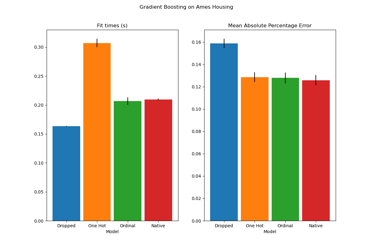
該圖顯示，對類別特徵的新本機支援導致的擬合時間與將類別視為有序量的模型相當，也就是簡單地進行序數編碼。本機支援也比單熱編碼和序數編碼更具表現力。但是，要使用新的 categorical_features 參數，仍然需要在管線中預處理資料，如此範例所示。

HistGradientBoosting 估計器的效能提升

在呼叫 fit 期間，ensemble.HistGradientBoostingRegressor 和 ensemble.HistGradientBoostingClassifier 的記憶體佔用量已顯著改善。此外，現在可以平行完成直方圖初始化，從而略微提高了速度。請在基準測試頁面中查看更多內容。

新的自訓練元估計器

基於 Yarowski 演算法的新自訓練實作現在可以與任何實作 predict_proba 的分類器搭配使用。子分類器將充當半監督分類器，使其能夠從未標記的資料中學習。請在使用者指南中閱讀更多內容。

import numpy as np
from sklearn import datasets
from sklearn.semi_supervised import SelfTrainingClassifier
from sklearn.svm import SVC

rng = np.random.RandomState(42)
iris = datasets.load_iris()
random_unlabeled_points = rng.rand(iris.target.shape[0]) < 0.3
iris.target[random_unlabeled_points] = -1
svc = SVC(probability=True, gamma="auto")
self_training_model = SelfTrainingClassifier(svc)
self_training_model.fit(iris.data, iris.target)

SelfTrainingClassifier(estimator=SVC(gamma='auto', probability=True))

在 Jupyter 環境中，請重新執行此儲存格以顯示 HTML 表示或信任筆記本。
在 GitHub 上，HTML 表示無法呈現，請嘗試使用 nbviewer.org 載入此頁面。

新的 SequentialFeatureSelector 轉換器

現在可以使用新的迭代轉換器來選擇特徵：SequentialFeatureSelector。序列特徵選擇可以根據交叉驗證的分數最大化，一次新增一個特徵（正向選擇）或從可用的特徵列表中刪除特徵（反向選擇）。請參閱使用者指南。

from sklearn.feature_selection import SequentialFeatureSelector
from sklearn.neighbors import KNeighborsClassifier
from sklearn.datasets import load_iris

X, y = load_iris(return_X_y=True, as_frame=True)
feature_names = X.columns
knn = KNeighborsClassifier(n_neighbors=3)
sfs = SequentialFeatureSelector(knn, n_features_to_select=2)
sfs.fit(X, y)
print(
    "Features selected by forward sequential selection: "
    f"{feature_names[sfs.get_support()].tolist()}"
)

Features selected by forward sequential selection: ['sepal length (cm)', 'petal width (cm)']

新的 PolynomialCountSketch 核近似函數

新的 PolynomialCountSketch 在與線性模型一起使用時，會近似特徵空間的多項式展開，但比 PolynomialFeatures 使用的記憶體少得多。

from sklearn.datasets import fetch_covtype
from sklearn.pipeline import make_pipeline
from sklearn.model_selection import train_test_split
from sklearn.preprocessing import MinMaxScaler
from sklearn.kernel_approximation import PolynomialCountSketch
from sklearn.linear_model import LogisticRegression

X, y = fetch_covtype(return_X_y=True)
pipe = make_pipeline(
    MinMaxScaler(),
    PolynomialCountSketch(degree=2, n_components=300),
    LogisticRegression(max_iter=1000),
)
X_train, X_test, y_train, y_test = train_test_split(
    X, y, train_size=5000, test_size=10000, random_state=42
)
pipe.fit(X_train, y_train).score(X_test, y_test)

0.7307

為了比較，以下是相同數據的線性基準分數

linear_baseline = make_pipeline(MinMaxScaler(), LogisticRegression(max_iter=1000))
linear_baseline.fit(X_train, y_train).score(X_test, y_test)

0.714

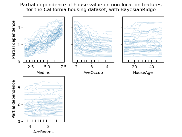
個別條件期望圖

現在可以使用一種新的部分依賴圖：個別條件期望 (Individual Conditional Expectation, ICE) 圖。ICE 圖以每條樣本一條線的方式，個別視覺化預測對每個樣本的特徵的依賴關係。請參閱使用者指南。

from sklearn.ensemble import RandomForestRegressor
from sklearn.datasets import fetch_california_housing

# from sklearn.inspection import plot_partial_dependence
from sklearn.inspection import PartialDependenceDisplay

X, y = fetch_california_housing(return_X_y=True, as_frame=True)
features = ["MedInc", "AveOccup", "HouseAge", "AveRooms"]
est = RandomForestRegressor(n_estimators=10)
est.fit(X, y)

# plot_partial_dependence has been removed in version 1.2. From 1.2, use
# PartialDependenceDisplay instead.
# display = plot_partial_dependence(
display = PartialDependenceDisplay.from_estimator(
    est,
    X,
    features,
    kind="individual",
    subsample=50,
    n_jobs=3,
    grid_resolution=20,
    random_state=0,
)
display.figure_.suptitle(
    "Partial dependence of house value on non-location features\n"
    "for the California housing dataset, with BayesianRidge"
)
display.figure_.subplots_adjust(hspace=0.3)

DecisionTreeRegressor 的新 Poisson 分裂準則

Poisson 迴歸估計的整合從 0.23 版本繼續。DecisionTreeRegressor 現在支援新的 'poisson' 分裂準則。如果您的目標是計數或頻率，設定 criterion="poisson" 可能是一個不錯的選擇。

from sklearn.tree import DecisionTreeRegressor
from sklearn.model_selection import train_test_split
import numpy as np

n_samples, n_features = 1000, 20
rng = np.random.RandomState(0)
X = rng.randn(n_samples, n_features)
# positive integer target correlated with X[:, 5] with many zeros:
y = rng.poisson(lam=np.exp(X[:, 5]) / 2)
X_train, X_test, y_train, y_test = train_test_split(X, y, random_state=rng)
regressor = DecisionTreeRegressor(criterion="poisson", random_state=0)
regressor.fit(X_train, y_train)

DecisionTreeRegressor(criterion='poisson', random_state=0)

在 Jupyter 環境中，請重新執行此儲存格以顯示 HTML 表示或信任筆記本。
在 GitHub 上，HTML 表示無法呈現，請嘗試使用 nbviewer.org 載入此頁面。

新的文件改進

新增了新的範例和文件頁面，以持續努力改進對機器學習實務的理解

• 關於常見陷阱和建議做法的新章節，

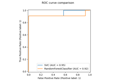
• 一個範例說明如何使用 GridSearchCV 評估的統計比較模型效能，

• 一個關於如何解釋線性模型係數的範例，

• 一個比較主成分迴歸和偏最小平方法的範例。

相關範例

scikit-learn 0.23 的發行重點

scikit-learn 0.23 的發行重點

scikit-learn 0.22 的發行重點

scikit-learn 0.22 的發行重點

scikit-learn 1.0 的發行重點

scikit-learn 1.0 的發行重點

scikit-learn 1.4 的發行重點

scikit-learn 1.4 的發行重點