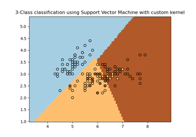
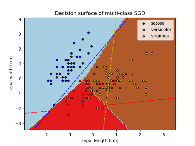
繪製在 iris 資料集上的多類別 SGD#

繪製 iris 資料集上多類別 SGD 的決策面。對應於三個一對多 (OVA) 分類器的超平面以虛線表示。

# Authors: The scikit-learn developers
# SPDX-License-Identifier: BSD-3-Clause

import matplotlib.pyplot as plt
import numpy as np

from sklearn import datasets
from sklearn.inspection import DecisionBoundaryDisplay
from sklearn.linear_model import SGDClassifier

# import some data to play with
iris = datasets.load_iris()

# we only take the first two features. We could
# avoid this ugly slicing by using a two-dim dataset
X = iris.data[:, :2]
y = iris.target
colors = "bry"

# shuffle
idx = np.arange(X.shape[0])
np.random.seed(13)
np.random.shuffle(idx)
X = X[idx]
y = y[idx]

# standardize
mean = X.mean(axis=0)
std = X.std(axis=0)
X = (X - mean) / std

clf = SGDClassifier(alpha=0.001, max_iter=100).fit(X, y)
ax = plt.gca()
DecisionBoundaryDisplay.from_estimator(
    clf,
    X,
    cmap=plt.cm.Paired,
    ax=ax,
    response_method="predict",
    xlabel=iris.feature_names[0],
    ylabel=iris.feature_names[1],
)
plt.axis("tight")

# Plot also the training points
for i, color in zip(clf.classes_, colors):
    idx = np.where(y == i)
    plt.scatter(
        X[idx, 0],
        X[idx, 1],
        c=color,
        label=iris.target_names[i],
        edgecolor="black",
        s=20,
    )
plt.title("Decision surface of multi-class SGD")
plt.axis("tight")

# Plot the three one-against-all classifiers
xmin, xmax = plt.xlim()
ymin, ymax = plt.ylim()
coef = clf.coef_
intercept = clf.intercept_


def plot_hyperplane(c, color):
    def line(x0):
        return (-(x0 * coef[c, 0]) - intercept[c]) / coef[c, 1]

    plt.plot([xmin, xmax], [line(xmin), line(xmax)], ls="--", color=color)


for i, color in zip(clf.classes_, colors):
    plot_hyperplane(i, color)
plt.legend()
plt.show()