注意
跳到末尾下載完整的範例程式碼。或透過 JupyterLite 或 Binder 在您的瀏覽器中執行此範例
k-means 假設的展示#
此範例旨在說明 k-means 產生不直觀且可能不希望的分群的情況。
# Authors: The scikit-learn developers
# SPDX-License-Identifier: BSD-3-Clause
資料產生#
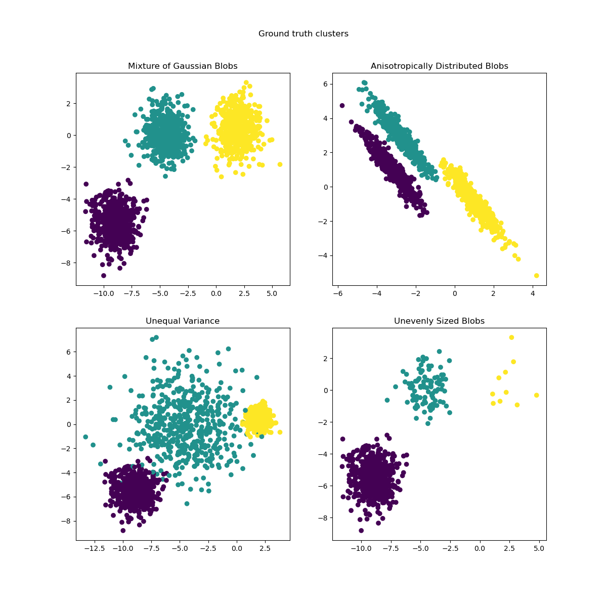
函數 make_blobs 產生等向性(球形)高斯斑點。若要獲得異向性(橢圓形)高斯斑點,必須定義線性 轉換。
import numpy as np

from sklearn.datasets import make_blobs

n_samples = 1500
random_state = 170
transformation = [[0.60834549, -0.63667341], [-0.40887718, 0.85253229]]

X, y = make_blobs(n_samples=n_samples, random_state=random_state)
X_aniso = np.dot(X, transformation)  # Anisotropic blobs
X_varied, y_varied = make_blobs(
    n_samples=n_samples, cluster_std=[1.0, 2.5, 0.5], random_state=random_state
)  # Unequal variance
X_filtered = np.vstack(
    (X[y == 0][:500], X[y == 1][:100], X[y == 2][:10])
)  # Unevenly sized blobs
y_filtered = [0] * 500 + [1] * 100 + [2] * 10
我們可以視覺化產生的資料
import matplotlib.pyplot as plt

fig, axs = plt.subplots(nrows=2, ncols=2, figsize=(12, 12))

axs[0, 0].scatter(X[:, 0], X[:, 1], c=y)
axs[0, 0].set_title("Mixture of Gaussian Blobs")

axs[0, 1].scatter(X_aniso[:, 0], X_aniso[:, 1], c=y)
axs[0, 1].set_title("Anisotropically Distributed Blobs")

axs[1, 0].scatter(X_varied[:, 0], X_varied[:, 1], c=y_varied)
axs[1, 0].set_title("Unequal Variance")

axs[1, 1].scatter(X_filtered[:, 0], X_filtered[:, 1], c=y_filtered)
axs[1, 1].set_title("Unevenly Sized Blobs")

plt.suptitle("Ground truth clusters").set_y(0.95)
plt.show()
擬合模型並繪製結果#
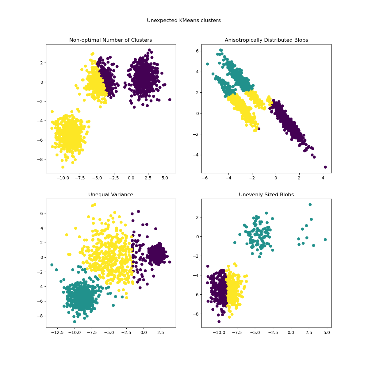
先前產生的資料現在用於顯示 KMeans 在以下情境中的行為
非最佳分群數:在真實設定中,沒有唯一定義的真實分群數。必須根據資料的準則和目標知識來決定適當的分群數。
異向性分佈的斑點:k-means 包括最小化樣本到其分配到的分群質心的歐幾里得距離。因此,k-means 更適用於等向性和常態分佈的分群(即球形高斯分佈)。
不等的變異數:k-means 等同於取得具有相同變異數但可能具有不同平均數的 k 高斯分佈的「混合」的最大似然估計量。
大小不均勻的斑點:沒有關於 k-means 的理論結果表明它需要相似的分群大小才能良好執行,但最小化歐幾里得距離確實意味著問題越稀疏且高維,就越需要使用不同的質心種子來執行演算法,以確保全域最小慣性。
from sklearn.cluster import KMeans

common_params = {
    "n_init": "auto",
    "random_state": random_state,
}

fig, axs = plt.subplots(nrows=2, ncols=2, figsize=(12, 12))

y_pred = KMeans(n_clusters=2, **common_params).fit_predict(X)
axs[0, 0].scatter(X[:, 0], X[:, 1], c=y_pred)
axs[0, 0].set_title("Non-optimal Number of Clusters")

y_pred = KMeans(n_clusters=3, **common_params).fit_predict(X_aniso)
axs[0, 1].scatter(X_aniso[:, 0], X_aniso[:, 1], c=y_pred)
axs[0, 1].set_title("Anisotropically Distributed Blobs")

y_pred = KMeans(n_clusters=3, **common_params).fit_predict(X_varied)
axs[1, 0].scatter(X_varied[:, 0], X_varied[:, 1], c=y_pred)
axs[1, 0].set_title("Unequal Variance")

y_pred = KMeans(n_clusters=3, **common_params).fit_predict(X_filtered)
axs[1, 1].scatter(X_filtered[:, 0], X_filtered[:, 1], c=y_pred)
axs[1, 1].set_title("Unevenly Sized Blobs")

plt.suptitle("Unexpected KMeans clusters").set_y(0.95)
plt.show()
可能的解決方案#
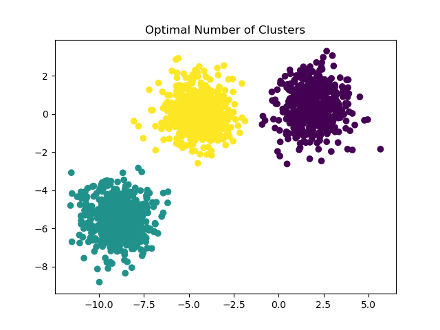
如需有關如何找到正確斑點數的範例,請參閱 在 KMeans 分群上使用輪廓分析選擇分群數。在此案例中,只需設定 n_clusters=3 即可。
y_pred = KMeans(n_clusters=3, **common_params).fit_predict(X)
plt.scatter(X[:, 0], X[:, 1], c=y_pred)
plt.title("Optimal Number of Clusters")
plt.show()
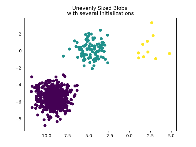
為了處理大小不均勻的斑點,可以增加隨機初始化的次數。在此案例中,我們設定 n_init=10 以避免找到次佳的局部最小值。如需更多詳細資訊,請參閱 使用 k-means 對稀疏資料進行分群。
y_pred = KMeans(n_clusters=3, n_init=10, random_state=random_state).fit_predict(
    X_filtered
)
plt.scatter(X_filtered[:, 0], X_filtered[:, 1], c=y_pred)
plt.title("Unevenly Sized Blobs \nwith several initializations")
plt.show()
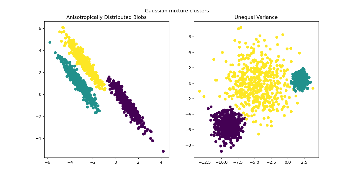
由於異向性和不等的變異數是 k-means 演算法的真正限制,因此我們在此建議改用 GaussianMixture,它也假設高斯分群,但不對其變異數施加任何限制。請注意,您仍然必須找到正確的斑點數(請參閱 高斯混合模型選擇)。
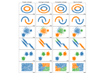
如需其他分群方法如何處理異向性或不等變異數斑點的範例,請參閱範例 比較玩具資料集上不同的分群演算法。
from sklearn.mixture import GaussianMixture

fig, (ax1, ax2) = plt.subplots(nrows=1, ncols=2, figsize=(12, 6))

y_pred = GaussianMixture(n_components=3).fit_predict(X_aniso)
ax1.scatter(X_aniso[:, 0], X_aniso[:, 1], c=y_pred)
ax1.set_title("Anisotropically Distributed Blobs")

y_pred = GaussianMixture(n_components=3).fit_predict(X_varied)
ax2.scatter(X_varied[:, 0], X_varied[:, 1], c=y_pred)
ax2.set_title("Unequal Variance")

plt.suptitle("Gaussian mixture clusters").set_y(0.95)
plt.show()
最終評論#
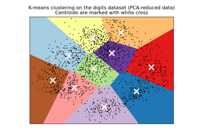
在高維空間中,歐幾里得距離往往會膨脹(此範例中未顯示)。在 k-means 分群之前執行降維演算法可以緩解此問題並加快計算速度(請參閱範例 使用 k-means 對文字文件進行分群)。
在已知分群是等向性、具有相似變異數且不太稀疏的情況下,k-means 演算法非常有效,並且是可用的最快分群演算法之一。如果必須重新啟動多次才能避免收斂到局部最小值,則此優勢將會喪失。
指令碼的總執行時間: (0 分鐘 1.145 秒)
相關範例