鄰域成分分析範例#

此範例說明了學習到的距離度量，該度量可最大化最近鄰分類準確性。它提供了此度量與原始點空間的視覺表示。請參閱使用者指南以獲取更多資訊。

# Authors: The scikit-learn developers
# SPDX-License-Identifier: BSD-3-Clause

import matplotlib.pyplot as plt
import numpy as np
from matplotlib import cm
from scipy.special import logsumexp

from sklearn.datasets import make_classification
from sklearn.neighbors import NeighborhoodComponentsAnalysis

原始點#

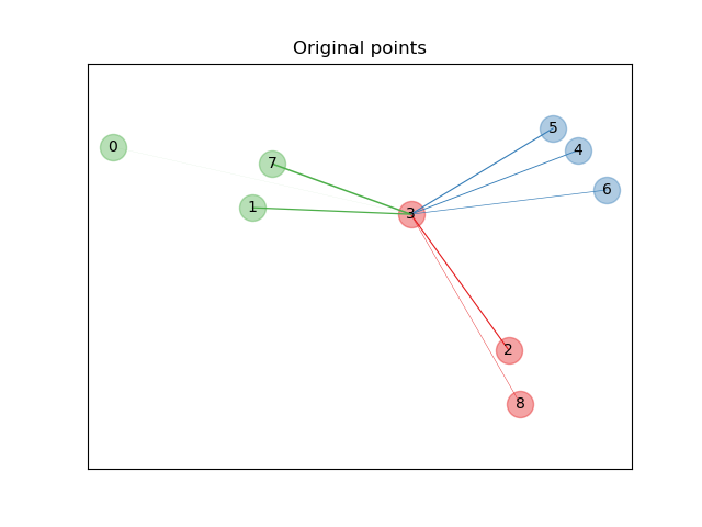
首先，我們建立一個包含來自 3 個類別的 9 個樣本的資料集，並在原始空間中繪製點。在此範例中，我們專注於第 3 個點的分類。第 3 個點與另一個點之間的連結厚度與它們的距離成正比。

X, y = make_classification(
    n_samples=9,
    n_features=2,
    n_informative=2,
    n_redundant=0,
    n_classes=3,
    n_clusters_per_class=1,
    class_sep=1.0,
    random_state=0,
)

plt.figure(1)
ax = plt.gca()
for i in range(X.shape[0]):
    ax.text(X[i, 0], X[i, 1], str(i), va="center", ha="center")
    ax.scatter(X[i, 0], X[i, 1], s=300, c=cm.Set1(y[[i]]), alpha=0.4)

ax.set_title("Original points")
ax.axes.get_xaxis().set_visible(False)
ax.axes.get_yaxis().set_visible(False)
ax.axis("equal")  # so that boundaries are displayed correctly as circles


def link_thickness_i(X, i):
    diff_embedded = X[i] - X
    dist_embedded = np.einsum("ij,ij->i", diff_embedded, diff_embedded)
    dist_embedded[i] = np.inf

    # compute exponentiated distances (use the log-sum-exp trick to
    # avoid numerical instabilities
    exp_dist_embedded = np.exp(-dist_embedded - logsumexp(-dist_embedded))
    return exp_dist_embedded


def relate_point(X, i, ax):
    pt_i = X[i]
    for j, pt_j in enumerate(X):
        thickness = link_thickness_i(X, i)
        if i != j:
            line = ([pt_i[0], pt_j[0]], [pt_i[1], pt_j[1]])
            ax.plot(*line, c=cm.Set1(y[j]), linewidth=5 * thickness[j])


i = 3
relate_point(X, i, ax)
plt.show()

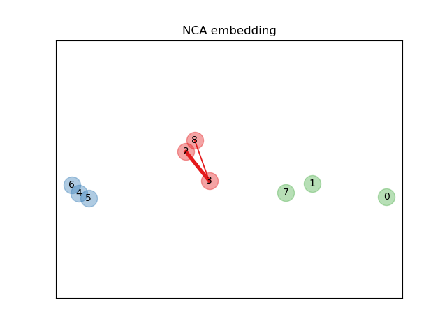
學習嵌入#

我們使用NeighborhoodComponentsAnalysis來學習嵌入，並在轉換後繪製點。然後，我們取得嵌入並找到最近鄰。

nca = NeighborhoodComponentsAnalysis(max_iter=30, random_state=0)
nca = nca.fit(X, y)

plt.figure(2)
ax2 = plt.gca()
X_embedded = nca.transform(X)
relate_point(X_embedded, i, ax2)

for i in range(len(X)):
    ax2.text(X_embedded[i, 0], X_embedded[i, 1], str(i), va="center", ha="center")
    ax2.scatter(X_embedded[i, 0], X_embedded[i, 1], s=300, c=cm.Set1(y[[i]]), alpha=0.4)

ax2.set_title("NCA embedding")
ax2.axes.get_xaxis().set_visible(False)
ax2.axes.get_yaxis().set_visible(False)
ax2.axis("equal")
plt.show()