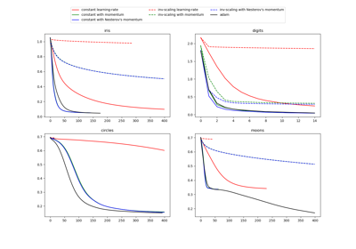
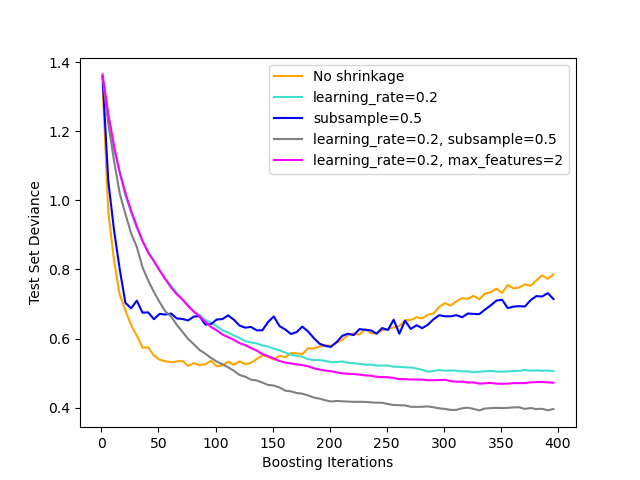
梯度提升正規化#

梯度提升不同正規化策略效果的說明。此範例取自 Hastie et al 2009 [1]。

使用的損失函數是二項偏差。透過收縮進行正規化 (learning_rate < 1.0) 可大幅提高效能。結合收縮，隨機梯度提升 (subsample < 1.0) 可以透過 Bagging 減少變異數，產生更準確的模型。不使用收縮的子抽樣通常效果不佳。另一種減少變異數的策略是透過子抽樣特徵，類似於隨機森林中的隨機拆分（透過 max_features 參數）。

# Authors: The scikit-learn developers
# SPDX-License-Identifier: BSD-3-Clause

import matplotlib.pyplot as plt
import numpy as np

from sklearn import datasets, ensemble
from sklearn.metrics import log_loss
from sklearn.model_selection import train_test_split

X, y = datasets.make_hastie_10_2(n_samples=4000, random_state=1)

# map labels from {-1, 1} to {0, 1}
labels, y = np.unique(y, return_inverse=True)

X_train, X_test, y_train, y_test = train_test_split(X, y, test_size=0.8, random_state=0)

original_params = {
    "n_estimators": 400,
    "max_leaf_nodes": 4,
    "max_depth": None,
    "random_state": 2,
    "min_samples_split": 5,
}

plt.figure()

for label, color, setting in [
    ("No shrinkage", "orange", {"learning_rate": 1.0, "subsample": 1.0}),
    ("learning_rate=0.2", "turquoise", {"learning_rate": 0.2, "subsample": 1.0}),
    ("subsample=0.5", "blue", {"learning_rate": 1.0, "subsample": 0.5}),
    (
        "learning_rate=0.2, subsample=0.5",
        "gray",
        {"learning_rate": 0.2, "subsample": 0.5},
    ),
    (
        "learning_rate=0.2, max_features=2",
        "magenta",
        {"learning_rate": 0.2, "max_features": 2},
    ),
]:
    params = dict(original_params)
    params.update(setting)

    clf = ensemble.GradientBoostingClassifier(**params)
    clf.fit(X_train, y_train)

    # compute test set deviance
    test_deviance = np.zeros((params["n_estimators"],), dtype=np.float64)

    for i, y_proba in enumerate(clf.staged_predict_proba(X_test)):
        test_deviance[i] = 2 * log_loss(y_test, y_proba[:, 1])

    plt.plot(
        (np.arange(test_deviance.shape[0]) + 1)[::5],
        test_deviance[::5],
        "-",
        color=color,
        label=label,
    )

plt.legend(loc="upper right")
plt.xlabel("Boosting Iterations")
plt.ylabel("Test Set Deviance")

plt.show()