注意
前往結尾下載完整的範例程式碼。或透過 JupyterLite 或 Binder 在您的瀏覽器中執行此範例
模型正規化對訓練和測試錯誤的影響#
在此範例中,我們評估名為 ElasticNet 的線性模型中正規化參數的影響。為了進行此評估,我們使用 ValidationCurveDisplay 使用驗證曲線。此曲線顯示模型對於不同正規化參數值的訓練和測試分數。
一旦我們確定最佳正規化參數,我們將比較模型的真實係數和估計係數,以確定模型是否能夠從雜訊輸入資料中恢復係數。
# Authors: The scikit-learn developers
# SPDX-License-Identifier: BSD-3-Clause
產生範例資料#
我們產生一個迴歸資料集,其中包含相對於樣本數量而言的許多特徵。但是,只有 10% 的特徵是有資訊的。在這種情況下,通常使用暴露 L1 懲罰的線性模型來恢復一組稀疏係數。
from sklearn.datasets import make_regression
from sklearn.model_selection import train_test_split

n_samples_train, n_samples_test, n_features = 150, 300, 500
X, y, true_coef = make_regression(
    n_samples=n_samples_train + n_samples_test,
    n_features=n_features,
    n_informative=50,
    shuffle=False,
    noise=1.0,
    coef=True,
    random_state=42,
)
X_train, X_test, y_train, y_test = train_test_split(
    X, y, train_size=n_samples_train, test_size=n_samples_test, shuffle=False
)
模型定義#
在這裡,我們不使用僅暴露 L1 懲罰的模型。相反,我們使用 ElasticNet 模型,該模型同時暴露 L1 和 L2 懲罰。
我們固定 l1_ratio 參數,以便模型找到的解仍然是稀疏的。因此,此類模型嘗試找到一個稀疏解,但同時也嘗試將所有係數縮小到零。
此外,我們強制模型的係數為正數,因為我們知道 make_regression 會產生具有正號的回應。因此,我們使用此預先知識來獲得更好的模型。
from sklearn.linear_model import ElasticNet

enet = ElasticNet(l1_ratio=0.9, positive=True, max_iter=10_000)
評估正規化參數的影響#
為了評估正規化參數的影響,我們使用驗證曲線。此曲線顯示模型對於不同正規化參數值的訓練和測試分數。
正規化 alpha 是應用於模型係數的參數:當它趨於零時,不應用正規化,模型嘗試以最小的誤差擬合訓練資料。但是,當特徵有雜訊時,會導致過擬合。當 alpha 增加時,模型係數受到約束,因此模型無法緊密擬合訓練資料,從而避免過擬合。但是,如果應用過多的正規化,則模型會欠擬合資料,並且無法正確捕獲訊號。
驗證曲線有助於找到兩者極端之間的良好平衡:模型沒有正規化,因此足夠靈活以擬合訊號,但又不會過於靈活以致過擬合。ValidationCurveDisplay 允許我們顯示整個 alpha 值範圍的訓練和驗證分數。
import numpy as np

from sklearn.model_selection import ValidationCurveDisplay

alphas = np.logspace(-5, 1, 60)
disp = ValidationCurveDisplay.from_estimator(
    enet,
    X_train,
    y_train,
    param_name="alpha",
    param_range=alphas,
    scoring="r2",
    n_jobs=2,
    score_type="both",
)
disp.ax_.set(
    title=r"Validation Curve for ElasticNet (R$^2$ Score)",
    xlabel=r"alpha (regularization strength)",
    ylabel="R$^2$ Score",
)

test_scores_mean = disp.test_scores.mean(axis=1)
idx_avg_max_test_score = np.argmax(test_scores_mean)
disp.ax_.vlines(
    alphas[idx_avg_max_test_score],
    disp.ax_.get_ylim()[0],
    test_scores_mean[idx_avg_max_test_score],
    color="k",
    linewidth=2,
    linestyle="--",
    label=f"Optimum on test\n$\\alpha$ = {alphas[idx_avg_max_test_score]:.2e}",
)
_ = disp.ax_.legend(loc="lower right")
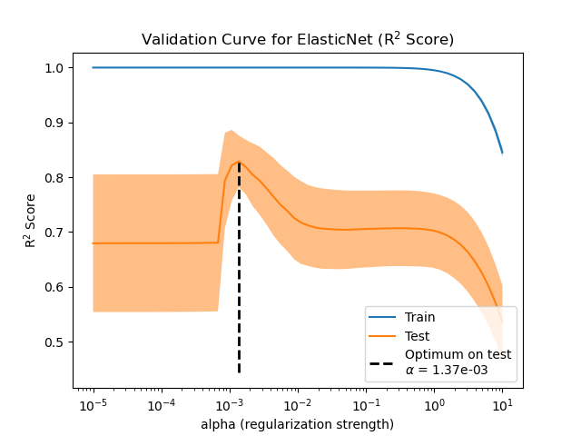
為了找到最佳正規化參數,我們可以選擇使驗證分數最大化的 alpha 值。
係數比較#
現在我們已經確定了最佳正規化參數,我們可以比較真實係數和估計係數。
首先,讓我們將正規化參數設定為最佳值,並將模型擬合到訓練資料上。此外,我們將顯示此模型的測試分數。
enet.set_params(alpha=alphas[idx_avg_max_test_score]).fit(X_train, y_train)
print(
    f"Test score: {enet.score(X_test, y_test):.3f}",
)
Test score: 0.884
現在,我們繪製真實係數和估計係數。
import matplotlib.pyplot as plt

fig, axs = plt.subplots(ncols=2, figsize=(12, 6), sharex=True, sharey=True)
for ax, coef, title in zip(axs, [true_coef, enet.coef_], ["True", "Model"]):
    ax.stem(coef)
    ax.set(
        title=f"{title} Coefficients",
        xlabel="Feature Index",
        ylabel="Coefficient Value",
    )
fig.suptitle(
    "Comparison of the coefficients of the true generative model and \n"
    "the estimated elastic net coefficients"
)

plt.show()
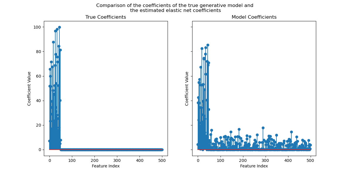
雖然原始係數是稀疏的,但估計係數並不那麼稀疏。原因在於我們將 l1_ratio 參數固定為 0.9。我們可以透過增加 l1_ratio 參數來強制模型獲得更稀疏的解。
但是,我們觀察到,對於真實生成模型中接近零的估計係數,我們的模型會將它們縮小到零。因此,我們沒有恢復真實係數,而是獲得了與測試集上獲得的效能一致的合理結果。
腳本的總執行時間:(0 分鐘 4.820 秒)
相關範例