注意
跳到結尾下載完整的範例程式碼。或透過 JupyterLite 或 Binder 在您的瀏覽器中執行此範例
核嶺迴歸和高斯過程迴歸的比較#
此範例說明了核嶺迴歸和高斯過程迴歸之間的差異。
核嶺迴歸和高斯過程迴歸都使用所謂的「核心技巧」,使其模型具有足夠的表現力來擬合訓練數據。然而,這兩種方法解決的機器學習問題截然不同。
核嶺迴歸會找到使損失函數(均方誤差)最小化的目標函數。
高斯過程迴歸不是找到單一目標函數,而是採用概率方法:基於貝氏定理定義目標函數上的高斯後驗分佈。因此,目標函數的先驗機率會與觀察到的訓練數據定義的可能性函數結合,以提供後驗分佈的估計值。
我們將透過一個範例來說明這些差異,並且我們也將專注於調整核心超參數。
# Authors: The scikit-learn developers
# SPDX-License-Identifier: BSD-3-Clause
產生資料集#
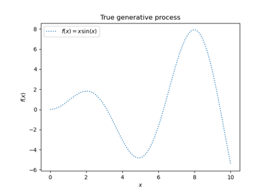
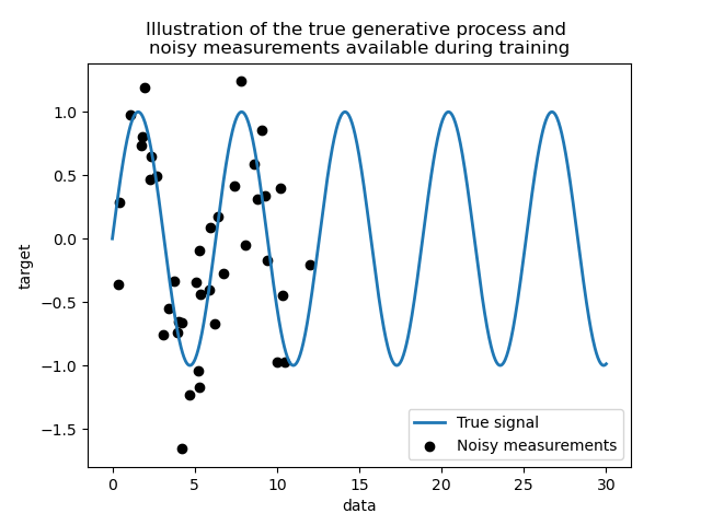
我們建立一個合成資料集。真正的產生過程會取一個 1 維向量並計算其正弦值。請注意,此正弦波的週期因此為 \(2 \pi\)。我們稍後將在此範例中重複使用此資訊。
import numpy as np

rng = np.random.RandomState(0)
data = np.linspace(0, 30, num=1_000).reshape(-1, 1)
target = np.sin(data).ravel()
現在,我們可以想像一個情境,我們從這個真實過程中獲得觀察結果。但是,我們將增加一些挑戰
測量結果會有雜訊;
僅提供訊號開始部分的樣本。
training_sample_indices = rng.choice(np.arange(0, 400), size=40, replace=False)
training_data = data[training_sample_indices]
training_noisy_target = target[training_sample_indices] + 0.5 * rng.randn(
    len(training_sample_indices)
)
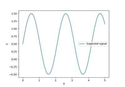
讓我們繪製真實訊號和可供訓練的雜訊測量結果。
import matplotlib.pyplot as plt

plt.plot(data, target, label="True signal", linewidth=2)
plt.scatter(
    training_data,
    training_noisy_target,
    color="black",
    label="Noisy measurements",
)
plt.legend()
plt.xlabel("data")
plt.ylabel("target")
_ = plt.title(
    "Illustration of the true generative process and \n"
    "noisy measurements available during training"
)
簡單線性模型的限制#
首先,我們想強調在給定資料集的情況下線性模型的限制。我們擬合一個 Ridge 並檢查此模型在我們資料集上的預測結果。
from sklearn.linear_model import Ridge

ridge = Ridge().fit(training_data, training_noisy_target)

plt.plot(data, target, label="True signal", linewidth=2)
plt.scatter(
    training_data,
    training_noisy_target,
    color="black",
    label="Noisy measurements",
)
plt.plot(data, ridge.predict(data), label="Ridge regression")
plt.legend()
plt.xlabel("data")
plt.ylabel("target")
_ = plt.title("Limitation of a linear model such as ridge")
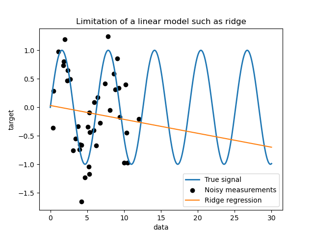
這種嶺迴歸器由於不夠具有表現力而欠擬合資料。
核心方法:核嶺和高斯過程#
核嶺#
我們可以透過使用所謂的核心來使先前的線性模型更具表現力。核心是從原始特徵空間到另一個特徵空間的嵌入。簡而言之,它用於將我們的原始數據映射到更新且更複雜的特徵空間。這個新的空間由核心的選擇明確定義。
在我們的例子中,我們知道真正的產生過程是一個週期性函數。我們可以使 ExpSineSquared 核心,它可以恢復週期性。類別 KernelRidge 將接受這樣一個核心。
將此模型與核心一起使用等效於使用核心的映射函數嵌入數據,然後應用嶺迴歸。在實踐中,數據不會被明確映射;而是使用「核心技巧」計算較高維特徵空間中樣本之間的點積。
因此,讓我們使用這樣一個 KernelRidge。
import time

from sklearn.gaussian_process.kernels import ExpSineSquared
from sklearn.kernel_ridge import KernelRidge

kernel_ridge = KernelRidge(kernel=ExpSineSquared())

start_time = time.time()
kernel_ridge.fit(training_data, training_noisy_target)
print(
    f"Fitting KernelRidge with default kernel: {time.time() - start_time:.3f} seconds"
)
Fitting KernelRidge with default kernel: 0.001 seconds
plt.plot(data, target, label="True signal", linewidth=2, linestyle="dashed")
plt.scatter(
    training_data,
    training_noisy_target,
    color="black",
    label="Noisy measurements",
)
plt.plot(
    data,
    kernel_ridge.predict(data),
    label="Kernel ridge",
    linewidth=2,
    linestyle="dashdot",
)
plt.legend(loc="lower right")
plt.xlabel("data")
plt.ylabel("target")
_ = plt.title(
    "Kernel ridge regression with an exponential sine squared\n "
    "kernel using default hyperparameters"
)
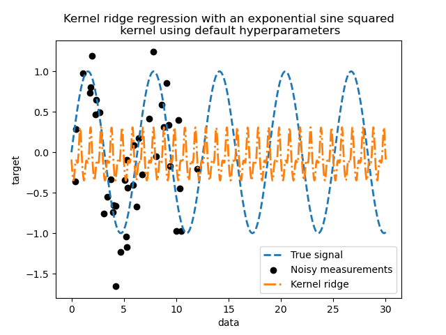
此擬合模型不準確。事實上,我們沒有設定核心的參數,而是使用了預設參數。我們可以檢查它們。
kernel_ridge.kernel
ExpSineSquared(length_scale=1, periodicity=1)
我們的核心有兩個參數:長度尺度和週期性。對於我們的資料集,我們使用 sin 作為產生過程,表示訊號的週期性為 \(2 \pi\)。參數的預設值為 \(1\),這解釋了我們模型預測中觀察到的高頻率。使用長度尺度參數可以得出類似的結論。因此,它告訴我們核心參數需要調整。我們將使用隨機搜尋來調整核心嶺模型的不同參數:alpha 參數和核心參數。
from scipy.stats import loguniform

from sklearn.model_selection import RandomizedSearchCV

param_distributions = {
    "alpha": loguniform(1e0, 1e3),
    "kernel__length_scale": loguniform(1e-2, 1e2),
    "kernel__periodicity": loguniform(1e0, 1e1),
}
kernel_ridge_tuned = RandomizedSearchCV(
    kernel_ridge,
    param_distributions=param_distributions,
    n_iter=500,
    random_state=0,
)
start_time = time.time()
kernel_ridge_tuned.fit(training_data, training_noisy_target)
print(f"Time for KernelRidge fitting: {time.time() - start_time:.3f} seconds")
Time for KernelRidge fitting: 4.240 seconds
由於我們必須嘗試多種超參數組合,因此現在擬合模型的計算成本更高。我們可以查看找到的超參數以獲得一些直覺。
kernel_ridge_tuned.best_params_
{'alpha': np.float64(1.991584977345022), 'kernel__length_scale': np.float64(0.7986499491396734), 'kernel__periodicity': np.float64(6.6072758064261095)}
查看最佳參數,我們看到它們與預設值不同。我們也看到週期性更接近預期值:\(2 \pi\)。我們現在可以檢查調整後的核嶺的預測。
Time for KernelRidge predict: 0.001 seconds
plt.plot(data, target, label="True signal", linewidth=2, linestyle="dashed")
plt.scatter(
    training_data,
    training_noisy_target,
    color="black",
    label="Noisy measurements",
)
plt.plot(
    data,
    predictions_kr,
    label="Kernel ridge",
    linewidth=2,
    linestyle="dashdot",
)
plt.legend(loc="lower right")
plt.xlabel("data")
plt.ylabel("target")
_ = plt.title(
    "Kernel ridge regression with an exponential sine squared\n "
    "kernel using tuned hyperparameters"
)
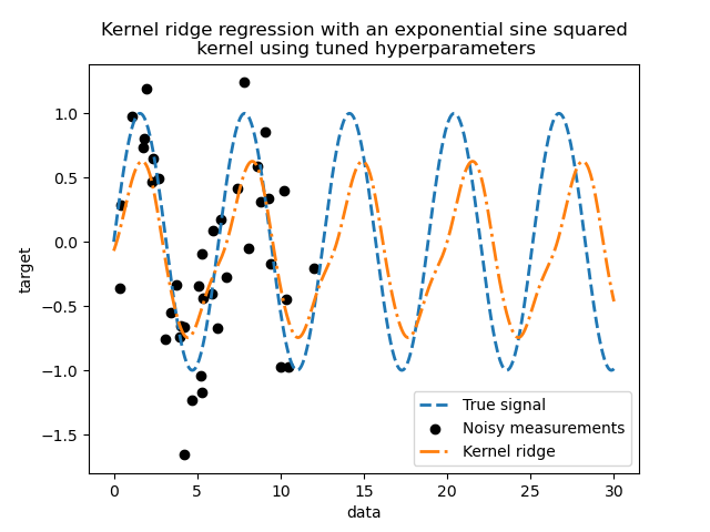
我們得到了一個更準確的模型。我們仍然觀察到一些錯誤,主要是由於添加到資料集的雜訊。
高斯過程迴歸#
現在,我們將使用 GaussianProcessRegressor 來擬合相同的資料集。在訓練高斯過程時,核心的超參數會在擬合過程中進行最佳化。無需進行外部超參數搜尋。在這裡,我們建立一個比核嶺迴歸器稍微複雜的核心:我們添加一個 WhiteKernel,用於估計資料集中的雜訊。
from sklearn.gaussian_process import GaussianProcessRegressor
from sklearn.gaussian_process.kernels import WhiteKernel

kernel = 1.0 * ExpSineSquared(1.0, 5.0, periodicity_bounds=(1e-2, 1e1)) + WhiteKernel(
    1e-1
)
gaussian_process = GaussianProcessRegressor(kernel=kernel)
start_time = time.time()
gaussian_process.fit(training_data, training_noisy_target)
print(
    f"Time for GaussianProcessRegressor fitting: {time.time() - start_time:.3f} seconds"
)
Time for GaussianProcessRegressor fitting: 0.030 seconds
訓練高斯過程的計算成本遠低於使用隨機搜尋的核嶺。我們可以檢查我們計算出的核心參數。
gaussian_process.kernel_
0.675**2 * ExpSineSquared(length_scale=1.34, periodicity=6.57) + WhiteKernel(noise_level=0.182)
事實上,我們看到參數已經最佳化。查看 periodicity 參數,我們看到我們找到了一個接近理論值 \(2 \pi\) 的週期。我們現在可以看看我們模型的預測。
Time for GaussianProcessRegressor predict: 0.002 seconds
plt.plot(data, target, label="True signal", linewidth=2, linestyle="dashed")
plt.scatter(
    training_data,
    training_noisy_target,
    color="black",
    label="Noisy measurements",
)
# Plot the predictions of the kernel ridge
plt.plot(
    data,
    predictions_kr,
    label="Kernel ridge",
    linewidth=2,
    linestyle="dashdot",
)
# Plot the predictions of the gaussian process regressor
plt.plot(
    data,
    mean_predictions_gpr,
    label="Gaussian process regressor",
    linewidth=2,
    linestyle="dotted",
)
plt.fill_between(
    data.ravel(),
    mean_predictions_gpr - std_predictions_gpr,
    mean_predictions_gpr + std_predictions_gpr,
    color="tab:green",
    alpha=0.2,
)
plt.legend(loc="lower right")
plt.xlabel("data")
plt.ylabel("target")
_ = plt.title("Comparison between kernel ridge and gaussian process regressor")
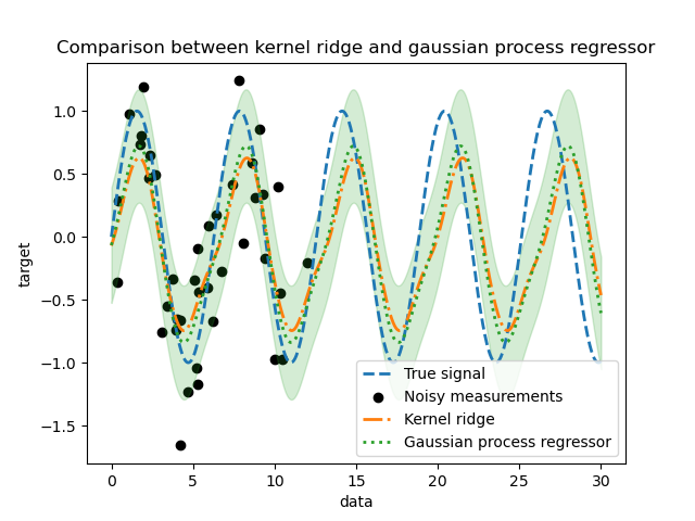
我們觀察到核嶺和高斯過程迴歸器的結果很接近。但是,高斯過程迴歸器還提供核嶺無法獲得的不確定性資訊。由於目標函數的概率公式,高斯過程可以輸出標準差(或共變異數)以及目標函數的平均預測。
但是,這是要付出代價的:使用高斯過程計算預測的時間更高。
最終結論#
我們可以就這兩個模型進行外推的可能性給出最後的結論。事實上,我們只提供了訊號的開頭作為訓練集。使用週期性核心會強制我們的模型重複在訓練集上找到的模式。將此核心資訊與這兩個模型的外推能力結合使用,我們觀察到這些模型將繼續預測正弦模式。
高斯過程允許將核心組合在一起。因此,我們可以將指數正弦平方核心與徑向基函數核心相關聯。
from sklearn.gaussian_process.kernels import RBF

kernel = 1.0 * ExpSineSquared(1.0, 5.0, periodicity_bounds=(1e-2, 1e1)) * RBF(
    length_scale=15, length_scale_bounds="fixed"
) + WhiteKernel(1e-1)
gaussian_process = GaussianProcessRegressor(kernel=kernel)
gaussian_process.fit(training_data, training_noisy_target)
mean_predictions_gpr, std_predictions_gpr = gaussian_process.predict(
    data,
    return_std=True,
)
plt.plot(data, target, label="True signal", linewidth=2, linestyle="dashed")
plt.scatter(
    training_data,
    training_noisy_target,
    color="black",
    label="Noisy measurements",
)
# Plot the predictions of the kernel ridge
plt.plot(
    data,
    predictions_kr,
    label="Kernel ridge",
    linewidth=2,
    linestyle="dashdot",
)
# Plot the predictions of the gaussian process regressor
plt.plot(
    data,
    mean_predictions_gpr,
    label="Gaussian process regressor",
    linewidth=2,
    linestyle="dotted",
)
plt.fill_between(
    data.ravel(),
    mean_predictions_gpr - std_predictions_gpr,
    mean_predictions_gpr + std_predictions_gpr,
    color="tab:green",
    alpha=0.2,
)
plt.legend(loc="lower right")
plt.xlabel("data")
plt.ylabel("target")
_ = plt.title("Effect of using a radial basis function kernel")
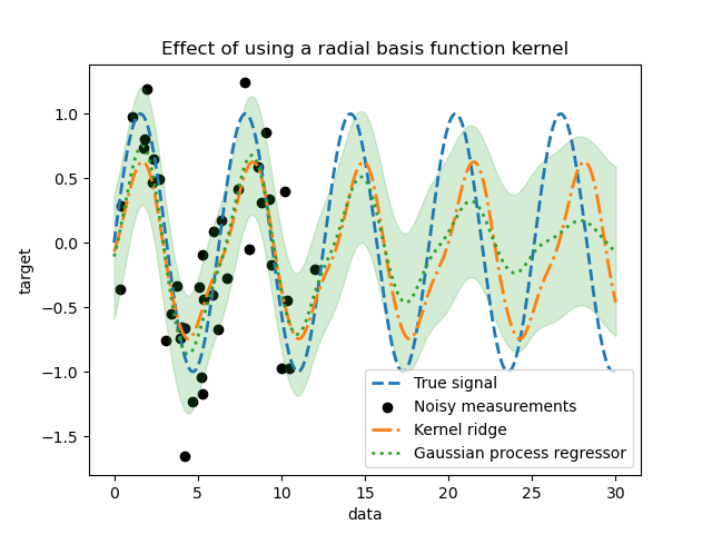
當訓練集中沒有樣本時,使用徑向基函數核(radial basis function kernel)會減弱週期性效應。隨著測試樣本與訓練樣本的距離越來越遠,預測值會趨於其平均值,並且其標準差也會增加。
腳本總執行時間: (0 分鐘 4.908 秒)
相關範例