手寫數字的流形學習：局部線性嵌入、Isomap…#

我們在數字資料集上說明各種嵌入技術。

# Authors: The scikit-learn developers
# SPDX-License-Identifier: BSD-3-Clause

載入數字資料集#

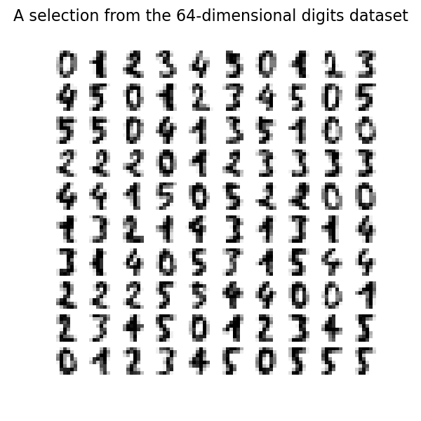
我們將載入數字資料集，並且只使用十個可用類別中的前六個類別。

from sklearn.datasets import load_digits

digits = load_digits(n_class=6)
X, y = digits.data, digits.target
n_samples, n_features = X.shape
n_neighbors = 30

我們可以繪製此資料集中的前一百個數字。

import matplotlib.pyplot as plt

fig, axs = plt.subplots(nrows=10, ncols=10, figsize=(6, 6))
for idx, ax in enumerate(axs.ravel()):
    ax.imshow(X[idx].reshape((8, 8)), cmap=plt.cm.binary)
    ax.axis("off")
_ = fig.suptitle("A selection from the 64-dimensional digits dataset", fontsize=16)

A selection from the 64-dimensional digits dataset

繪製嵌入的輔助函數#

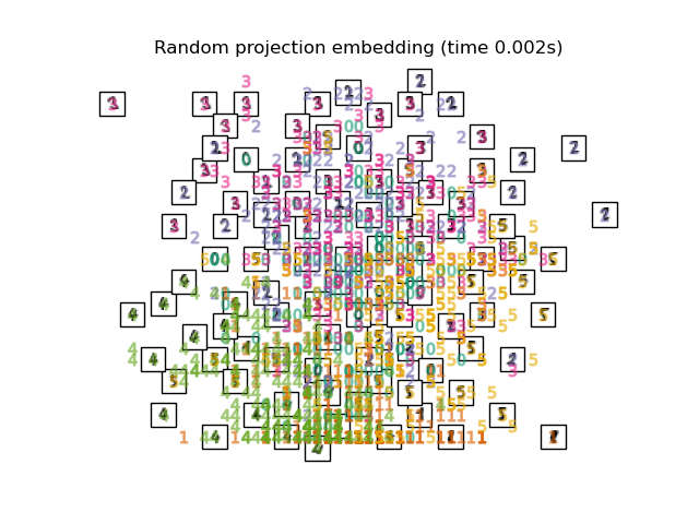
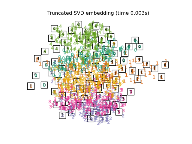
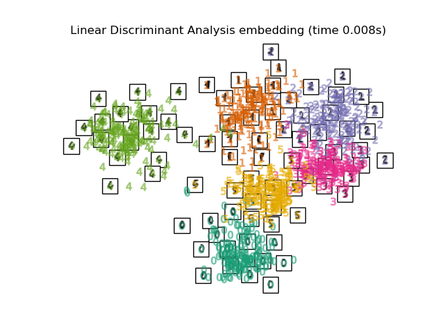
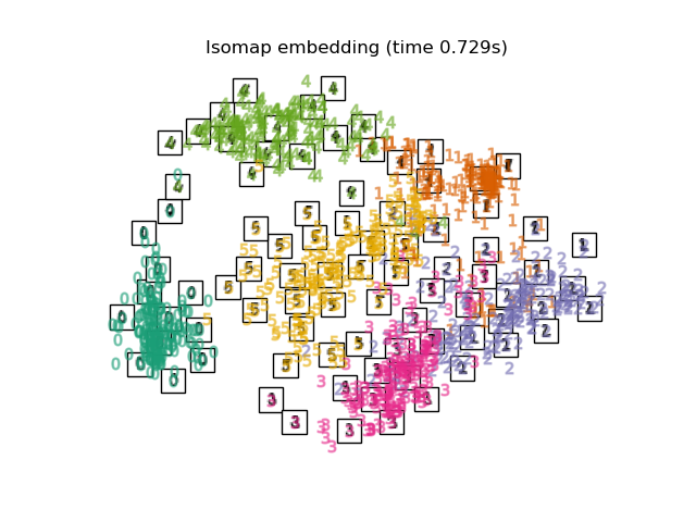
在下面，我們將使用不同的技術來嵌入數字資料集。我們將繪製原始資料在每個嵌入上的投影。這將允許我們檢查數字是否在嵌入空間中群組在一起，或是分散在其上。

import numpy as np
from matplotlib import offsetbox

from sklearn.preprocessing import MinMaxScaler


def plot_embedding(X, title):
    _, ax = plt.subplots()
    X = MinMaxScaler().fit_transform(X)

    for digit in digits.target_names:
        ax.scatter(
            *X[y == digit].T,
            marker=f"${digit}$",
            s=60,
            color=plt.cm.Dark2(digit),
            alpha=0.425,
            zorder=2,
        )
    shown_images = np.array([[1.0, 1.0]])  # just something big
    for i in range(X.shape[0]):
        # plot every digit on the embedding
        # show an annotation box for a group of digits
        dist = np.sum((X[i] - shown_images) ** 2, 1)
        if np.min(dist) < 4e-3:
            # don't show points that are too close
            continue
        shown_images = np.concatenate([shown_images, [X[i]]], axis=0)
        imagebox = offsetbox.AnnotationBbox(
            offsetbox.OffsetImage(digits.images[i], cmap=plt.cm.gray_r), X[i]
        )
        imagebox.set(zorder=1)
        ax.add_artist(imagebox)

    ax.set_title(title)
    ax.axis("off")

嵌入技術比較#

在下面，我們比較不同的技術。但是，有幾件事需要注意

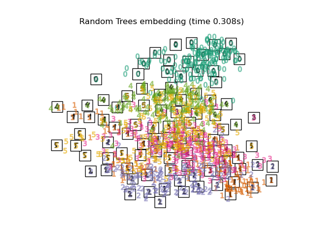
RandomTreesEmbedding 在技術上不是流形嵌入方法，因為它學習高維表示，我們在該表示上應用降維方法。但是，將資料集轉換為類別可線性分離的表示通常很有用。
LinearDiscriminantAnalysis 和 NeighborhoodComponentsAnalysis 是監督式降維方法，即它們使用提供的標籤，這與其他方法相反。
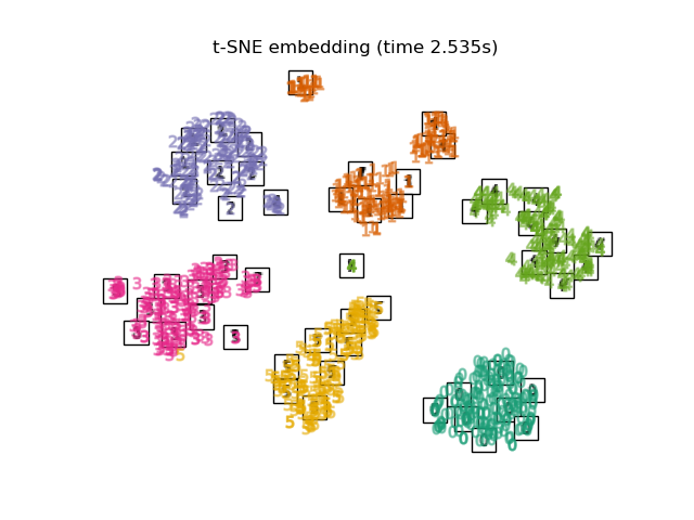
在此範例中，TSNE 是使用 PCA 產生的嵌入初始化。它確保嵌入的整體穩定性，即嵌入不依賴於隨機初始化。

from sklearn.decomposition import TruncatedSVD
from sklearn.discriminant_analysis import LinearDiscriminantAnalysis
from sklearn.ensemble import RandomTreesEmbedding
from sklearn.manifold import (
    MDS,
    TSNE,
    Isomap,
    LocallyLinearEmbedding,
    SpectralEmbedding,
)
from sklearn.neighbors import NeighborhoodComponentsAnalysis
from sklearn.pipeline import make_pipeline
from sklearn.random_projection import SparseRandomProjection

embeddings = {
    "Random projection embedding": SparseRandomProjection(
        n_components=2, random_state=42
    ),
    "Truncated SVD embedding": TruncatedSVD(n_components=2),
    "Linear Discriminant Analysis embedding": LinearDiscriminantAnalysis(
        n_components=2
    ),
    "Isomap embedding": Isomap(n_neighbors=n_neighbors, n_components=2),
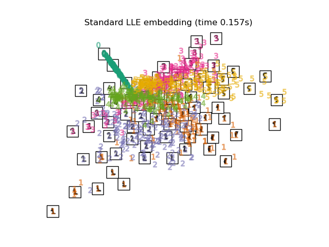
    "Standard LLE embedding": LocallyLinearEmbedding(
        n_neighbors=n_neighbors, n_components=2, method="standard"
    ),
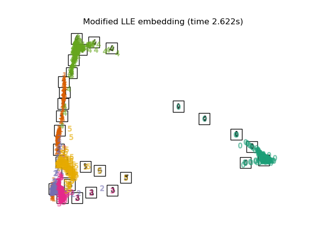
    "Modified LLE embedding": LocallyLinearEmbedding(
        n_neighbors=n_neighbors, n_components=2, method="modified"
    ),
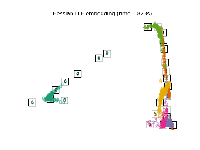
    "Hessian LLE embedding": LocallyLinearEmbedding(
        n_neighbors=n_neighbors, n_components=2, method="hessian"
    ),
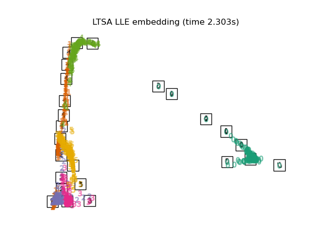
    "LTSA LLE embedding": LocallyLinearEmbedding(
        n_neighbors=n_neighbors, n_components=2, method="ltsa"
    ),
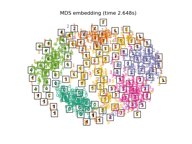
    "MDS embedding": MDS(n_components=2, n_init=1, max_iter=120, n_jobs=2),
    "Random Trees embedding": make_pipeline(
        RandomTreesEmbedding(n_estimators=200, max_depth=5, random_state=0),
        TruncatedSVD(n_components=2),
    ),
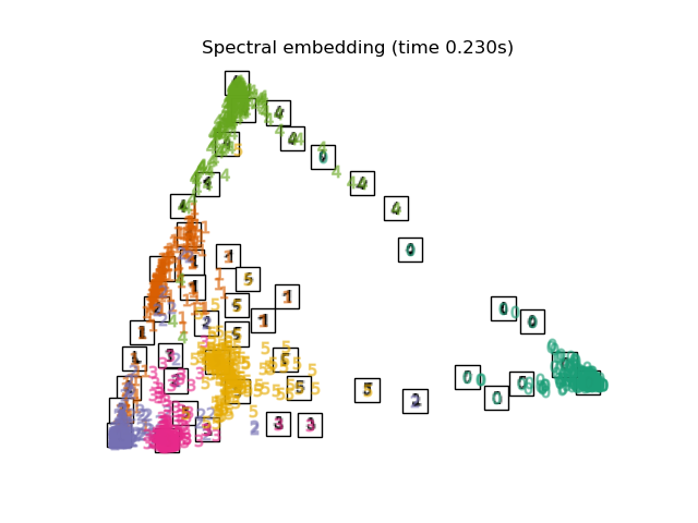
    "Spectral embedding": SpectralEmbedding(
        n_components=2, random_state=0, eigen_solver="arpack"
    ),
    "t-SNE embedding": TSNE(
        n_components=2,
        max_iter=500,
        n_iter_without_progress=150,
        n_jobs=2,
        random_state=0,
    ),
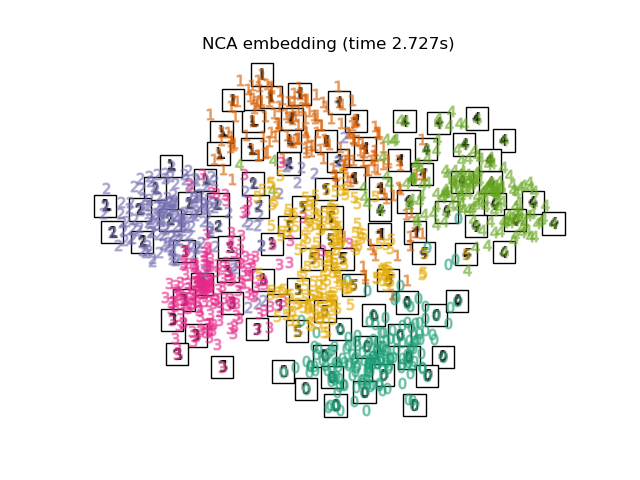
    "NCA embedding": NeighborhoodComponentsAnalysis(
        n_components=2, init="pca", random_state=0
    ),
}

一旦我們宣告了所有感興趣的方法，我們就可以執行並執行原始資料的投影。我們將儲存投影的資料以及執行每個投影所需的計算時間。

from time import time

projections, timing = {}, {}
for name, transformer in embeddings.items():
    if name.startswith("Linear Discriminant Analysis"):
        data = X.copy()
        data.flat[:: X.shape[1] + 1] += 0.01  # Make X invertible
    else:
        data = X

    print(f"Computing {name}...")
    start_time = time()
    projections[name] = transformer.fit_transform(data, y)
    timing[name] = time() - start_time

Computing Random projection embedding...
Computing Truncated SVD embedding...
Computing Linear Discriminant Analysis embedding...
Computing Isomap embedding...
Computing Standard LLE embedding...
Computing Modified LLE embedding...
Computing Hessian LLE embedding...
Computing LTSA LLE embedding...
Computing MDS embedding...
Computing Random Trees embedding...
Computing Spectral embedding...
Computing t-SNE embedding...
Computing NCA embedding...

最後，我們可以繪製每種方法給出的結果投影。

for name in timing:
    title = f"{name} (time {timing[name]:.3f}s)"
    plot_embedding(projections[name], title)

plt.show()

腳本總執行時間： (0 分鐘 20.718 秒)

相關範例