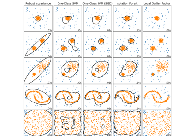
IsolationForest 範例#

使用 IsolationForest 進行異常偵測的範例。

Isolation Forest 是一個「隔離樹」的集成，透過遞迴隨機分割來「隔離」觀察值，可以用樹狀結構表示。隔離樣本所需的分割數對於離群值較低，對於內群值較高。

在本範例中，我們示範兩種視覺化在玩具數據集上訓練的 Isolation Forest 的決策邊界的方法。

# Authors: The scikit-learn developers
# SPDX-License-Identifier: BSD-3-Clause

數據產生#

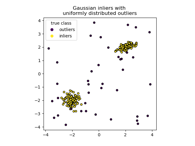
我們透過隨機採樣由 numpy.random.randn 返回的標準常態分佈，生成兩個叢集（每個叢集包含 n_samples）。其中一個是球形的，另一個則略微變形。

為了與 IsolationForest 符號一致，內群值（即高斯叢集）會被分配一個真實標籤 1，而離群值（使用 numpy.random.uniform 創建）則被分配標籤 -1。

import numpy as np

from sklearn.model_selection import train_test_split

n_samples, n_outliers = 120, 40
rng = np.random.RandomState(0)
covariance = np.array([[0.5, -0.1], [0.7, 0.4]])
cluster_1 = 0.4 * rng.randn(n_samples, 2) @ covariance + np.array([2, 2])  # general
cluster_2 = 0.3 * rng.randn(n_samples, 2) + np.array([-2, -2])  # spherical
outliers = rng.uniform(low=-4, high=4, size=(n_outliers, 2))

X = np.concatenate([cluster_1, cluster_2, outliers])
y = np.concatenate(
    [np.ones((2 * n_samples), dtype=int), -np.ones((n_outliers), dtype=int)]
)

X_train, X_test, y_train, y_test = train_test_split(X, y, stratify=y, random_state=42)

我們可以視覺化產生的叢集

import matplotlib.pyplot as plt

scatter = plt.scatter(X[:, 0], X[:, 1], c=y, s=20, edgecolor="k")
handles, labels = scatter.legend_elements()
plt.axis("square")
plt.legend(handles=handles, labels=["outliers", "inliers"], title="true class")
plt.title("Gaussian inliers with \nuniformly distributed outliers")
plt.show()

Gaussian inliers with uniformly distributed outliers

模型訓練#

from sklearn.ensemble import IsolationForest

clf = IsolationForest(max_samples=100, random_state=0)
clf.fit(X_train)

IsolationForest(max_samples=100, random_state=0)

在 Jupyter 環境中，請重新執行此單元格以顯示 HTML 表示，或信任筆記本。
在 GitHub 上，HTML 表示無法呈現，請嘗試使用 nbviewer.org 加載此頁面。

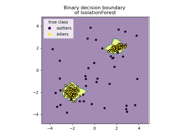
繪製離散決策邊界#

我們使用 DecisionBoundaryDisplay 類別來視覺化離散決策邊界。背景顏色表示預測給定區域中的樣本是否為離群值。散點圖顯示真實標籤。

import matplotlib.pyplot as plt

from sklearn.inspection import DecisionBoundaryDisplay

disp = DecisionBoundaryDisplay.from_estimator(
    clf,
    X,
    response_method="predict",
    alpha=0.5,
)
disp.ax_.scatter(X[:, 0], X[:, 1], c=y, s=20, edgecolor="k")
disp.ax_.set_title("Binary decision boundary \nof IsolationForest")
plt.axis("square")
plt.legend(handles=handles, labels=["outliers", "inliers"], title="true class")
plt.show()

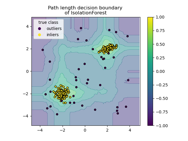
Binary decision boundary of IsolationForest

繪製路徑長度決策邊界#

透過設定 response_method="decision_function"，DecisionBoundaryDisplay 的背景表示觀察值的常態性度量。此類分數由隨機樹森林平均的路徑長度給出，而路徑長度本身由隔離給定樣本所需的葉子深度（或等效的分割次數）給出。

當隨機樹森林集體產生用於隔離某些特定樣本的短路徑長度時，它們很有可能成為異常值，並且常態性度量接近 0。同樣地，長路徑對應於接近 1 的值，並且更有可能為內群值。

disp = DecisionBoundaryDisplay.from_estimator(
    clf,
    X,
    response_method="decision_function",
    alpha=0.5,
)
disp.ax_.scatter(X[:, 0], X[:, 1], c=y, s=20, edgecolor="k")
disp.ax_.set_title("Path length decision boundary \nof IsolationForest")
plt.axis("square")
plt.legend(handles=handles, labels=["outliers", "inliers"], title="true class")
plt.colorbar(disp.ax_.collections[1])
plt.show()