注意
移至結尾以下載完整的範例程式碼。或透過 JupyterLite 或 Binder 在您的瀏覽器中執行此範例
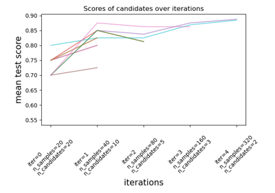
網格搜尋與連續減半之間的比較#
此範例比較了 HalvingGridSearchCV 和 GridSearchCV 所執行的參數搜尋。
# Authors: The scikit-learn developers
# SPDX-License-Identifier: BSD-3-Clause

from time import time

import matplotlib.pyplot as plt
import numpy as np
import pandas as pd

from sklearn import datasets
from sklearn.experimental import enable_halving_search_cv  # noqa
from sklearn.model_selection import GridSearchCV, HalvingGridSearchCV
from sklearn.svm import SVC
我們首先為 SVC 估計器定義參數空間,並計算訓練 HalvingGridSearchCV 實例以及 GridSearchCV 實例所需的時間。
rng = np.random.RandomState(0)
X, y = datasets.make_classification(n_samples=1000, random_state=rng)

gammas = [1e-1, 1e-2, 1e-3, 1e-4, 1e-5, 1e-6, 1e-7]
Cs = [1, 10, 100, 1e3, 1e4, 1e5]
param_grid = {"gamma": gammas, "C": Cs}

clf = SVC(random_state=rng)

tic = time()
gsh = HalvingGridSearchCV(
    estimator=clf, param_grid=param_grid, factor=2, random_state=rng
)
gsh.fit(X, y)
gsh_time = time() - tic

tic = time()
gs = GridSearchCV(estimator=clf, param_grid=param_grid)
gs.fit(X, y)
gs_time = time() - tic
我們現在繪製兩個搜尋估計器的熱圖。
def make_heatmap(ax, gs, is_sh=False, make_cbar=False):
    """Helper to make a heatmap."""
    results = pd.DataFrame(gs.cv_results_)
    results[["param_C", "param_gamma"]] = results[["param_C", "param_gamma"]].astype(
        np.float64
    )
    if is_sh:
        # SH dataframe: get mean_test_score values for the highest iter
        scores_matrix = results.sort_values("iter").pivot_table(
            index="param_gamma",
            columns="param_C",
            values="mean_test_score",
            aggfunc="last",
        )
    else:
        scores_matrix = results.pivot(
            index="param_gamma", columns="param_C", values="mean_test_score"
        )

    im = ax.imshow(scores_matrix)

    ax.set_xticks(np.arange(len(Cs)))
    ax.set_xticklabels(["{:.0E}".format(x) for x in Cs])
    ax.set_xlabel("C", fontsize=15)

    ax.set_yticks(np.arange(len(gammas)))
    ax.set_yticklabels(["{:.0E}".format(x) for x in gammas])
    ax.set_ylabel("gamma", fontsize=15)

    # Rotate the tick labels and set their alignment.
    plt.setp(ax.get_xticklabels(), rotation=45, ha="right", rotation_mode="anchor")

    if is_sh:
        iterations = results.pivot_table(
            index="param_gamma", columns="param_C", values="iter", aggfunc="max"
        ).values
        for i in range(len(gammas)):
            for j in range(len(Cs)):
                ax.text(
                    j,
                    i,
                    iterations[i, j],
                    ha="center",
                    va="center",
                    color="w",
                    fontsize=20,
                )

    if make_cbar:
        fig.subplots_adjust(right=0.8)
        cbar_ax = fig.add_axes([0.85, 0.15, 0.05, 0.7])
        fig.colorbar(im, cax=cbar_ax)
        cbar_ax.set_ylabel("mean_test_score", rotation=-90, va="bottom", fontsize=15)


fig, axes = plt.subplots(ncols=2, sharey=True)
ax1, ax2 = axes

make_heatmap(ax1, gsh, is_sh=True)
make_heatmap(ax2, gs, make_cbar=True)

ax1.set_title("Successive Halving\ntime = {:.3f}s".format(gsh_time), fontsize=15)
ax2.set_title("GridSearch\ntime = {:.3f}s".format(gs_time), fontsize=15)

plt.show()
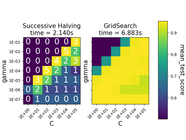
熱圖顯示 SVC 實例的參數組合的平均測試分數。HalvingGridSearchCV 也顯示上次使用組合的疊代。標記為 0 的組合僅在第一次疊代中評估,而標記為 5 的組合則是認為最佳的參數組合。
我們可以發現 HalvingGridSearchCV 類別能夠找到與 GridSearchCV 一樣準確的參數組合,而且花費的時間更少。
腳本的總執行時間: (0 分鐘 9.206 秒)
相關範例