注意
前往結尾以下載完整的範例程式碼。或透過 JupyterLite 或 Binder 在您的瀏覽器中執行此範例
梯度提升中的類別特徵支援#
在此範例中,我們將比較 HistGradientBoostingRegressor 針對類別特徵使用不同編碼策略的訓練時間和預測效能。特別是,我們將評估
捨棄類別特徵
使用
OrdinalEncoder並將類別視為有序的、等距的量使用
OrdinalEncoder並依賴 原生類別支援 的HistGradientBoostingRegressor估計器。
我們將使用 Ames Iowa Housing 資料集,其中包含數值和類別特徵,房屋的銷售價格為目標。
請參閱 直方圖梯度提升樹中的特徵,以取得展示 HistGradientBoostingRegressor 其他特徵的範例。
# Authors: The scikit-learn developers
# SPDX-License-Identifier: BSD-3-Clause
載入 Ames Housing 資料集#
首先,我們將 Ames Housing 資料載入為 pandas 資料框架。這些特徵分為類別或數值
from sklearn.datasets import fetch_openml

X, y = fetch_openml(data_id=42165, as_frame=True, return_X_y=True)

# Select only a subset of features of X to make the example faster to run
categorical_columns_subset = [
    "BldgType",
    "GarageFinish",
    "LotConfig",
    "Functional",
    "MasVnrType",
    "HouseStyle",
    "FireplaceQu",
    "ExterCond",
    "ExterQual",
    "PoolQC",
]

numerical_columns_subset = [
    "3SsnPorch",
    "Fireplaces",
    "BsmtHalfBath",
    "HalfBath",
    "GarageCars",
    "TotRmsAbvGrd",
    "BsmtFinSF1",
    "BsmtFinSF2",
    "GrLivArea",
    "ScreenPorch",
]

X = X[categorical_columns_subset + numerical_columns_subset]
X[categorical_columns_subset] = X[categorical_columns_subset].astype("category")

categorical_columns = X.select_dtypes(include="category").columns
n_categorical_features = len(categorical_columns)
n_numerical_features = X.select_dtypes(include="number").shape[1]

print(f"Number of samples: {X.shape[0]}")
print(f"Number of features: {X.shape[1]}")
print(f"Number of categorical features: {n_categorical_features}")
print(f"Number of numerical features: {n_numerical_features}")
Number of samples: 1460
Number of features: 20
Number of categorical features: 10
Number of numerical features: 10
具有捨棄類別特徵的梯度提升估計器#
作為基準,我們建立一個會捨棄類別特徵的估計器
from sklearn.compose import make_column_selector, make_column_transformer
from sklearn.ensemble import HistGradientBoostingRegressor
from sklearn.pipeline import make_pipeline

dropper = make_column_transformer(
    ("drop", make_column_selector(dtype_include="category")), remainder="passthrough"
)
hist_dropped = make_pipeline(dropper, HistGradientBoostingRegressor(random_state=42))
具有獨熱編碼的梯度提升估計器#
接下來,我們建立一個管道,該管道會獨熱編碼類別特徵,並讓其餘的數值資料通過
from sklearn.preprocessing import OneHotEncoder

one_hot_encoder = make_column_transformer(
    (
        OneHotEncoder(sparse_output=False, handle_unknown="ignore"),
        make_column_selector(dtype_include="category"),
    ),
    remainder="passthrough",
)

hist_one_hot = make_pipeline(
    one_hot_encoder, HistGradientBoostingRegressor(random_state=42)
)
具有序數編碼的梯度提升估計器#
接下來,我們建立一個管道,該管道會將類別特徵視為有序的量,也就是說,類別將編碼為 0、1、2 等,並視為連續特徵。
import numpy as np

from sklearn.preprocessing import OrdinalEncoder

ordinal_encoder = make_column_transformer(
    (
        OrdinalEncoder(handle_unknown="use_encoded_value", unknown_value=np.nan),
        make_column_selector(dtype_include="category"),
    ),
    remainder="passthrough",
    # Use short feature names to make it easier to specify the categorical
    # variables in the HistGradientBoostingRegressor in the next step
    # of the pipeline.
    verbose_feature_names_out=False,
)

hist_ordinal = make_pipeline(
    ordinal_encoder, HistGradientBoostingRegressor(random_state=42)
)
具有原生類別支援的梯度提升估計器#
現在,我們建立一個將原生處理類別特徵的 HistGradientBoostingRegressor 估計器。此估計器不會將類別特徵視為有序的量。我們設定 categorical_features="from_dtype",以便將具有類別 dtype 的特徵視為類別特徵。
此估計器與前一個估計器之間的主要差異在於,在此估計器中,我們讓 HistGradientBoostingRegressor 從 DataFrame 資料行的 dtypes 偵測哪些特徵是類別的。
hist_native = HistGradientBoostingRegressor(
    random_state=42, categorical_features="from_dtype"
)
模型比較#
最後,我們使用交叉驗證來評估模型。在此,我們比較模型在 mean_absolute_percentage_error 和擬合時間方面的效能。
import matplotlib.pyplot as plt

from sklearn.model_selection import cross_validate

scoring = "neg_mean_absolute_percentage_error"
n_cv_folds = 3

dropped_result = cross_validate(hist_dropped, X, y, cv=n_cv_folds, scoring=scoring)
one_hot_result = cross_validate(hist_one_hot, X, y, cv=n_cv_folds, scoring=scoring)
ordinal_result = cross_validate(hist_ordinal, X, y, cv=n_cv_folds, scoring=scoring)
native_result = cross_validate(hist_native, X, y, cv=n_cv_folds, scoring=scoring)


def plot_results(figure_title):
    fig, (ax1, ax2) = plt.subplots(1, 2, figsize=(12, 8))

    plot_info = [
        ("fit_time", "Fit times (s)", ax1, None),
        ("test_score", "Mean Absolute Percentage Error", ax2, None),
    ]

    x, width = np.arange(4), 0.9
    for key, title, ax, y_limit in plot_info:
        items = [
            dropped_result[key],
            one_hot_result[key],
            ordinal_result[key],
            native_result[key],
        ]

        mape_cv_mean = [np.mean(np.abs(item)) for item in items]
        mape_cv_std = [np.std(item) for item in items]

        ax.bar(
            x=x,
            height=mape_cv_mean,
            width=width,
            yerr=mape_cv_std,
            color=["C0", "C1", "C2", "C3"],
        )
        ax.set(
            xlabel="Model",
            title=title,
            xticks=x,
            xticklabels=["Dropped", "One Hot", "Ordinal", "Native"],
            ylim=y_limit,
        )
    fig.suptitle(figure_title)


plot_results("Gradient Boosting on Ames Housing")
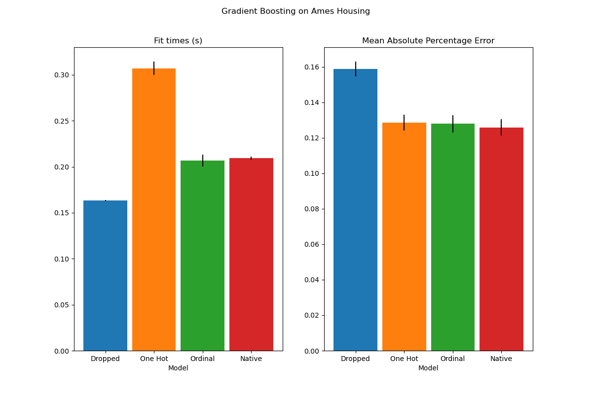
我們看到,具有獨熱編碼資料的模型是目前最慢的。這是預期的,因為獨熱編碼會為每個類別值(針對每個類別特徵)建立一個額外的特徵,因此在擬合期間需要考慮更多分割點。理論上,我們預期原生處理類別特徵會比將類別視為有序量 ('Ordinal') 稍微慢一些,因為原生處理需要排序類別。然而,當類別數量很少時,擬合時間應該會很接近,而且這可能不總是在實務中反映出來。
在預測效能方面,捨棄類別特徵會導致較差的效能。使用類別特徵的三個模型的錯誤率相當,原生處理略勝一籌。
限制分割數#
一般而言,可以預期從獨熱編碼資料中獲得較差的預測,尤其是當樹的深度或節點數有限時:使用獨熱編碼資料時,需要更多分割點(即更深的深度)才能恢復原生處理在單一分割點中可以獲得的等效分割。
當類別被視為序數量時也是如此:如果類別是 A..F,而最佳分割是 ACF - BDE,則獨熱編碼模型需要 3 個分割點(左節點中每個類別一個分割點),而序數非原生模型需要 4 個分割:1 個分割以隔離 A,1 個分割以隔離 F,以及 2 個分割以從 BCDE 中隔離 C。
模型效能在實務上的差異有多大取決於資料集和樹的彈性。
為了看到這一點,讓我們重新執行相同的分析,使用欠擬合模型,我們透過限制樹的數量和每棵樹的深度來人為地限制分割總數。
for pipe in (hist_dropped, hist_one_hot, hist_ordinal, hist_native):
    if pipe is hist_native:
        # The native model does not use a pipeline so, we can set the parameters
        # directly.
        pipe.set_params(max_depth=3, max_iter=15)
    else:
        pipe.set_params(
            histgradientboostingregressor__max_depth=3,
            histgradientboostingregressor__max_iter=15,
        )

dropped_result = cross_validate(hist_dropped, X, y, cv=n_cv_folds, scoring=scoring)
one_hot_result = cross_validate(hist_one_hot, X, y, cv=n_cv_folds, scoring=scoring)
ordinal_result = cross_validate(hist_ordinal, X, y, cv=n_cv_folds, scoring=scoring)
native_result = cross_validate(hist_native, X, y, cv=n_cv_folds, scoring=scoring)

plot_results("Gradient Boosting on Ames Housing (few and small trees)")

plt.show()
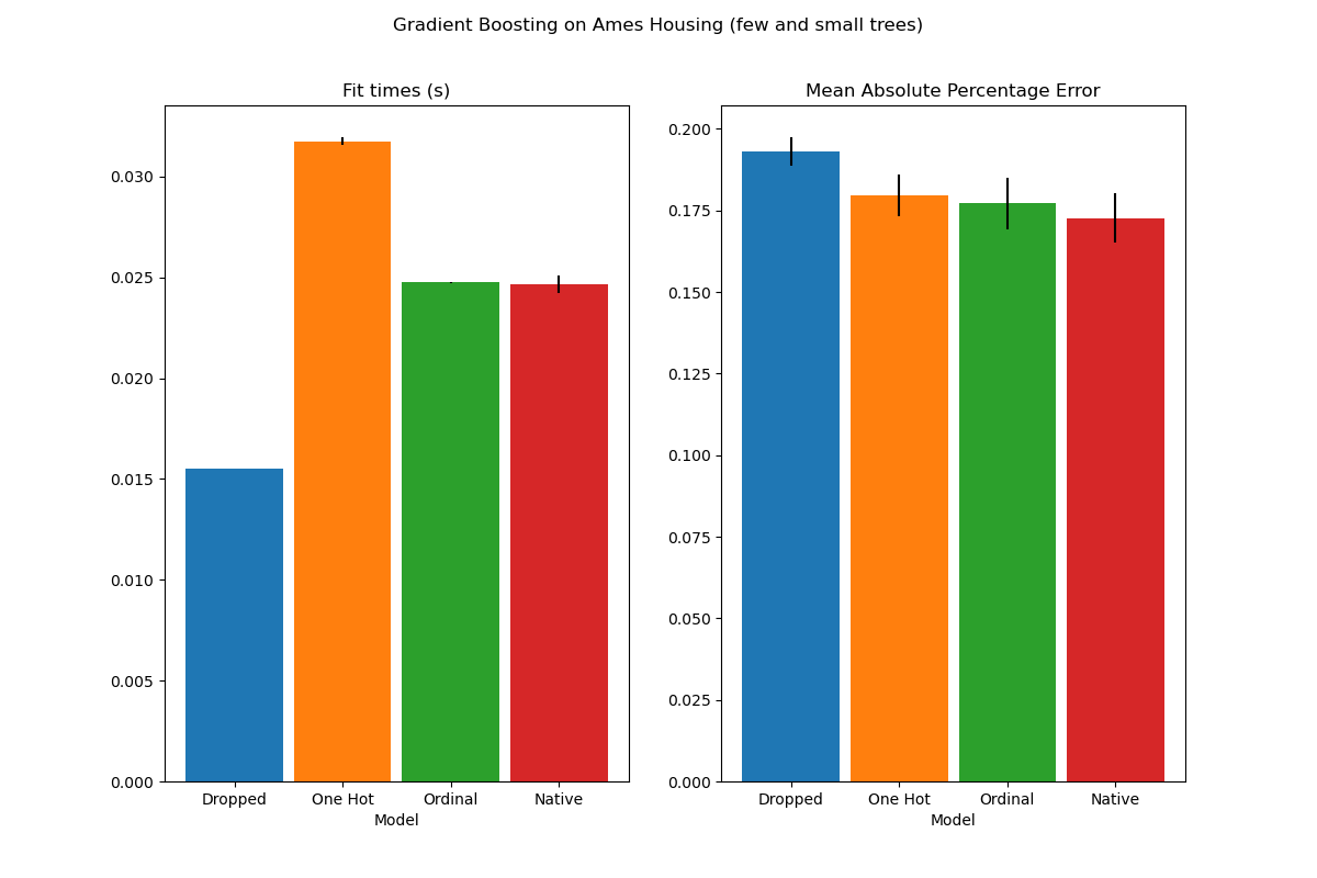
這些欠擬合模型的結果證實了我們先前的直覺:當分割預算受到限制時,原生類別處理策略的效能最佳。另外兩種策略(獨熱編碼和將類別視為序數值)導致的錯誤值與完全捨棄類別特徵的基準模型相當。
腳本的總執行時間:(0 分鐘 3.502 秒)
相關範例