注意
前往結尾以下載完整的範例程式碼。或透過 JupyterLite 或 Binder 在您的瀏覽器中執行此範例
比較線性貝氏迴歸器#
此範例比較兩個不同的貝氏迴歸器
一個 貝氏嶺迴歸
在第一部分中,我們使用普通最小平方法(OLS) 模型作為基準,以比較模型相對於真實係數的係數。之後,我們展示了此類模型的估計是透過迭代最大化觀測值的邊際對數可能性來完成的。
在最後一部分,我們使用多項式特徵擴展來繪製 ARD 和貝氏嶺迴歸的預測和不確定性,以擬合 X 和 y 之間的非線性關係。
# Authors: The scikit-learn developers
# SPDX-License-Identifier: BSD-3-Clause
模型恢復真實權重的穩健性#
產生合成資料集#
我們產生一個資料集,其中 X 和 y 線性關聯:X 的 10 個特徵將用於產生 y。其他特徵在預測 y 時沒有用處。此外,我們產生一個資料集,其中 n_samples == n_features。這種設定對於 OLS 模型來說具有挑戰性,並且可能導致任意大的權重。對權重和懲罰設定先驗可以緩解此問題。最後,會加入高斯雜訊。
from sklearn.datasets import make_regression

X, y, true_weights = make_regression(
    n_samples=100,
    n_features=100,
    n_informative=10,
    noise=8,
    coef=True,
    random_state=42,
)
擬合迴歸器#
我們現在擬合貝氏模型和 OLS,以便稍後比較模型的係數。
import pandas as pd

from sklearn.linear_model import ARDRegression, BayesianRidge, LinearRegression

olr = LinearRegression().fit(X, y)
brr = BayesianRidge(compute_score=True, max_iter=30).fit(X, y)
ard = ARDRegression(compute_score=True, max_iter=30).fit(X, y)
df = pd.DataFrame(
    {
        "Weights of true generative process": true_weights,
        "ARDRegression": ard.coef_,
        "BayesianRidge": brr.coef_,
        "LinearRegression": olr.coef_,
    }
)
繪製真實和估計的係數#
現在我們將每個模型的係數與真實生成模型的權重進行比較。
import matplotlib.pyplot as plt
import seaborn as sns
from matplotlib.colors import SymLogNorm

plt.figure(figsize=(10, 6))
ax = sns.heatmap(
    df.T,
    norm=SymLogNorm(linthresh=10e-4, vmin=-80, vmax=80),
    cbar_kws={"label": "coefficients' values"},
    cmap="seismic_r",
)
plt.ylabel("linear model")
plt.xlabel("coefficients")
plt.tight_layout(rect=(0, 0, 1, 0.95))
_ = plt.title("Models' coefficients")
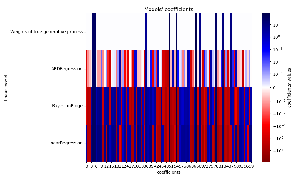
由於加入的雜訊,沒有一個模型能恢復真實的權重。實際上,所有模型始終都有超過 10 個非零係數。與 OLS 估計器相比,使用貝氏嶺迴歸的係數稍微向零偏移,這使得它們更穩定。ARD 迴歸提供了更稀疏的解:一些不提供資訊的係數被精確地設定為零,同時將其他係數偏移到更接近零。一些不提供資訊的係數仍然存在並保留較大的值。
繪製邊際對數可能性#
import numpy as np

ard_scores = -np.array(ard.scores_)
brr_scores = -np.array(brr.scores_)
plt.plot(ard_scores, color="navy", label="ARD")
plt.plot(brr_scores, color="red", label="BayesianRidge")
plt.ylabel("Log-likelihood")
plt.xlabel("Iterations")
plt.xlim(1, 30)
plt.legend()
_ = plt.title("Models log-likelihood")
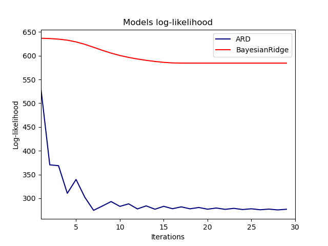
事實上,這兩個模型都將對數可能性最小化到由 max_iter 參數定義的任意截斷值。
使用多項式特徵擴展的貝氏迴歸#
產生合成資料集#
我們建立一個目標,它是輸入特徵的非線性函數。加入遵循標準均勻分佈的雜訊。
from sklearn.pipeline import make_pipeline
from sklearn.preprocessing import PolynomialFeatures, StandardScaler

rng = np.random.RandomState(0)
n_samples = 110

# sort the data to make plotting easier later
X = np.sort(-10 * rng.rand(n_samples) + 10)
noise = rng.normal(0, 1, n_samples) * 1.35
y = np.sqrt(X) * np.sin(X) + noise
full_data = pd.DataFrame({"input_feature": X, "target": y})
X = X.reshape((-1, 1))

# extrapolation
X_plot = np.linspace(10, 10.4, 10)
y_plot = np.sqrt(X_plot) * np.sin(X_plot)
X_plot = np.concatenate((X, X_plot.reshape((-1, 1))))
y_plot = np.concatenate((y - noise, y_plot))
擬合迴歸器#
這裡我們嘗試 10 次多項式來可能過度擬合,儘管貝氏線性模型會正規化多項式係數的大小。由於 ARDRegression 和 BayesianRidge 預設為 fit_intercept=True,因此 PolynomialFeatures 不應引入額外的偏差特徵。透過設定 return_std=True,貝氏迴歸器會傳回模型參數後驗分佈的標準差。
ard_poly = make_pipeline(
    PolynomialFeatures(degree=10, include_bias=False),
    StandardScaler(),
    ARDRegression(),
).fit(X, y)
brr_poly = make_pipeline(
    PolynomialFeatures(degree=10, include_bias=False),
    StandardScaler(),
    BayesianRidge(),
).fit(X, y)

y_ard, y_ard_std = ard_poly.predict(X_plot, return_std=True)
y_brr, y_brr_std = brr_poly.predict(X_plot, return_std=True)
繪製具有分數標準誤差的多項式迴歸#
ax = sns.scatterplot(
    data=full_data, x="input_feature", y="target", color="black", alpha=0.75
)
ax.plot(X_plot, y_plot, color="black", label="Ground Truth")
ax.plot(X_plot, y_brr, color="red", label="BayesianRidge with polynomial features")
ax.plot(X_plot, y_ard, color="navy", label="ARD with polynomial features")
ax.fill_between(
    X_plot.ravel(),
    y_ard - y_ard_std,
    y_ard + y_ard_std,
    color="navy",
    alpha=0.3,
)
ax.fill_between(
    X_plot.ravel(),
    y_brr - y_brr_std,
    y_brr + y_brr_std,
    color="red",
    alpha=0.3,
)
ax.legend()
_ = ax.set_title("Polynomial fit of a non-linear feature")
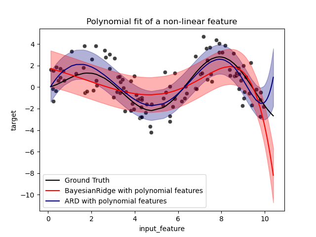
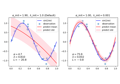
誤差條表示查詢點預測高斯分佈的一個標準差。請注意,當在兩個模型中使用預設參數時,ARD 迴歸最能捕捉到真實情況,但是進一步降低貝氏嶺迴歸的 lambda_init 超參數可以降低其偏差 (請參閱範例 使用貝氏嶺迴歸的曲線擬合)。最後,由於多項式迴歸的固有限制,這兩個模型在外推時都會失敗。
腳本的總執行時間: (0 分鐘 0.714 秒)
相關範例