使用多項式核心近似的可擴展學習#

此範例說明如何使用 PolynomialCountSketch 有效生成多項式核心特徵空間近似。這用於訓練線性分類器，以近似核心化分類器的準確性。

我們使用 Covtype 數據集 [2]，嘗試重現 Tensor Sketch [1] 原始論文中的實驗，即 PolynomialCountSketch 實作的演算法。

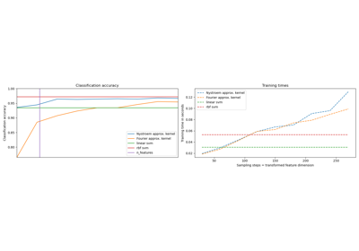
首先，我們計算原始特徵上線性分類器的準確性。然後，我們在由 PolynomialCountSketch 生成的不同數量特徵（n_components）上訓練線性分類器，以可擴展的方式近似核心化分類器的準確性。

# Authors: The scikit-learn developers
# SPDX-License-Identifier: BSD-3-Clause

準備數據#

載入 Covtype 數據集，其中包含 581,012 個樣本，每個樣本有 54 個特徵，分佈在 6 個類別中。此數據集的目標是僅從製圖變數（沒有遙感數據）預測森林覆蓋類型。載入後，我們將其轉換為二元分類問題，以匹配 LIBSVM 網頁 [2] 中數據集的版本，這是 [1] 中使用的版本。

from sklearn.datasets import fetch_covtype

X, y = fetch_covtype(return_X_y=True)

y[y != 2] = 0
y[y == 2] = 1  # We will try to separate class 2 from the other 6 classes.

分割數據#

這裡我們選擇 5,000 個樣本進行訓練，10,000 個樣本進行測試。要實際重現原始 Tensor Sketch 論文中的結果，請選擇 100,000 個進行訓練。

from sklearn.model_selection import train_test_split

X_train, X_test, y_train, y_test = train_test_split(
    X, y, train_size=5_000, test_size=10_000, random_state=42
)

特徵正規化#

現在將特徵縮放到 [0, 1] 範圍以匹配 LIBSVM 網頁中數據集的格式，然後如原始 Tensor Sketch 論文 [1] 中所做的那樣正規化為單位長度。

from sklearn.pipeline import make_pipeline
from sklearn.preprocessing import MinMaxScaler, Normalizer

mm = make_pipeline(MinMaxScaler(), Normalizer())
X_train = mm.fit_transform(X_train)
X_test = mm.transform(X_test)

建立基準模型#

作為基準，在原始特徵上訓練線性 SVM 並印出準確性。我們也測量並儲存準確性和訓練時間，以便稍後繪製它們。

import time

from sklearn.svm import LinearSVC

results = {}

lsvm = LinearSVC()
start = time.time()
lsvm.fit(X_train, y_train)
lsvm_time = time.time() - start
lsvm_score = 100 * lsvm.score(X_test, y_test)

results["LSVM"] = {"time": lsvm_time, "score": lsvm_score}
print(f"Linear SVM score on raw features: {lsvm_score:.2f}%")

Linear SVM score on raw features: 75.62%

建立核心近似模型#

然後，我們在由 PolynomialCountSketch 生成的特徵上訓練線性 SVM，並為 n_components 使用不同的值，顯示這些核心特徵近似提高了線性分類的準確性。在典型的應用場景中，n_components 應該大於輸入表示中的特徵數量，才能相對於線性分類實現改進。根據經驗，評估分數/運行時間成本的最佳值通常在 n_components = 10 * n_features 左右實現，儘管這可能取決於正在處理的特定數據集。請注意，由於原始樣本有 54 個特徵，因此四次多項式核心的顯式特徵映射大約有 850 萬個特徵（準確地說，54^4）。感謝 PolynomialCountSketch，我們可以將該特徵空間的大部分判別資訊濃縮到更緊湊的表示中。雖然我們在這個範例中只執行一次實驗（n_runs = 1），但在實務上，應該重複實驗幾次，以補償 PolynomialCountSketch 的隨機性質。

from sklearn.kernel_approximation import PolynomialCountSketch

n_runs = 1
N_COMPONENTS = [250, 500, 1000, 2000]

for n_components in N_COMPONENTS:
    ps_lsvm_time = 0
    ps_lsvm_score = 0
    for _ in range(n_runs):
        pipeline = make_pipeline(
            PolynomialCountSketch(n_components=n_components, degree=4),
            LinearSVC(),
        )

        start = time.time()
        pipeline.fit(X_train, y_train)
        ps_lsvm_time += time.time() - start
        ps_lsvm_score += 100 * pipeline.score(X_test, y_test)

    ps_lsvm_time /= n_runs
    ps_lsvm_score /= n_runs

    results[f"LSVM + PS({n_components})"] = {
        "time": ps_lsvm_time,
        "score": ps_lsvm_score,
    }
    print(
        f"Linear SVM score on {n_components} PolynomialCountSketch "
        + f"features: {ps_lsvm_score:.2f}%"
    )

Linear SVM score on 250 PolynomialCountSketch features: 76.55%
Linear SVM score on 500 PolynomialCountSketch features: 76.92%
Linear SVM score on 1000 PolynomialCountSketch features: 77.79%
Linear SVM score on 2000 PolynomialCountSketch features: 78.59%

建立核心化 SVM 模型#

訓練核心化 SVM 以查看 PolynomialCountSketch 如何近似核心的效能。當然，這可能需要一些時間，因為 SVC 類的擴展性相對較差。這就是核心近似器如此有用的原因

from sklearn.svm import SVC

ksvm = SVC(C=500.0, kernel="poly", degree=4, coef0=0, gamma=1.0)

start = time.time()
ksvm.fit(X_train, y_train)
ksvm_time = time.time() - start
ksvm_score = 100 * ksvm.score(X_test, y_test)

results["KSVM"] = {"time": ksvm_time, "score": ksvm_score}
print(f"Kernel-SVM score on raw features: {ksvm_score:.2f}%")

Kernel-SVM score on raw features: 79.78%

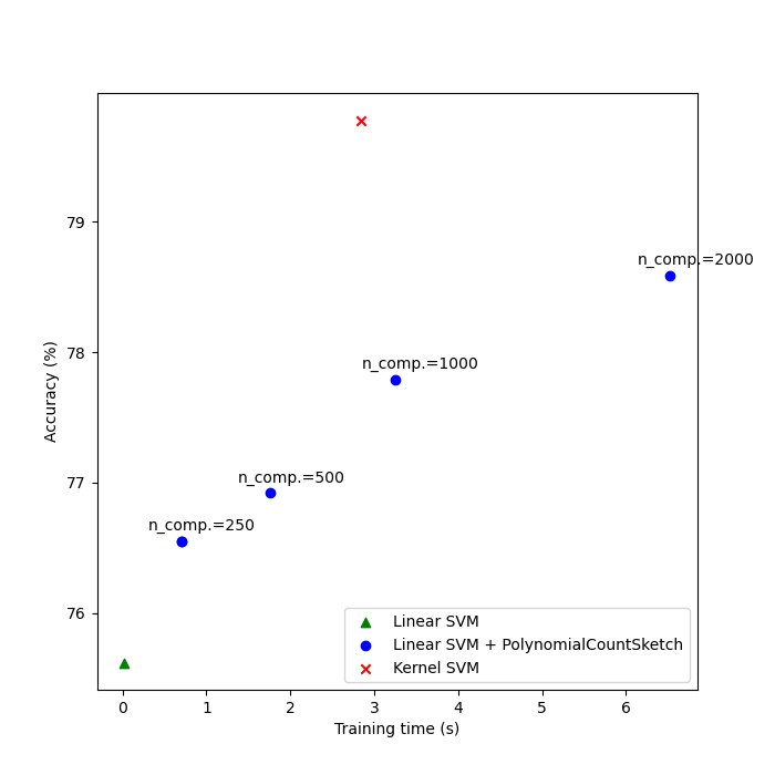
比較結果#

最後，繪製不同方法對其訓練時間的結果。正如我們所見，核心化 SVM 實現了更高的準確性，但其訓練時間要長得多，而且最重要的是，如果訓練樣本的數量增加，其訓練時間將會增長得更快。

import matplotlib.pyplot as plt

fig, ax = plt.subplots(figsize=(7, 7))
ax.scatter(
    [
        results["LSVM"]["time"],
    ],
    [
        results["LSVM"]["score"],
    ],
    label="Linear SVM",
    c="green",
    marker="^",
)

ax.scatter(
    [
        results["LSVM + PS(250)"]["time"],
    ],
    [
        results["LSVM + PS(250)"]["score"],
    ],
    label="Linear SVM + PolynomialCountSketch",
    c="blue",
)

for n_components in N_COMPONENTS:
    ax.scatter(
        [
            results[f"LSVM + PS({n_components})"]["time"],
        ],
        [
            results[f"LSVM + PS({n_components})"]["score"],
        ],
        c="blue",
    )
    ax.annotate(
        f"n_comp.={n_components}",
        (
            results[f"LSVM + PS({n_components})"]["time"],
            results[f"LSVM + PS({n_components})"]["score"],
        ),
        xytext=(-30, 10),
        textcoords="offset pixels",
    )

ax.scatter(
    [
        results["KSVM"]["time"],
    ],
    [
        results["KSVM"]["score"],
    ],
    label="Kernel SVM",
    c="red",
    marker="x",
)

ax.set_xlabel("Training time (s)")
ax.set_ylabel("Accuracy (%)")
ax.legend()
plt.show()