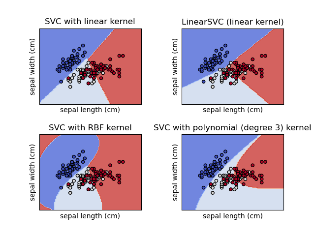
繪製 iris 資料集中不同的 SVM 分類器#

在 iris 資料集的 2D 投影上比較不同的線性 SVM 分類器。我們僅考慮此資料集的前 2 個特徵

萼片長度
萼片寬度

這個範例展示如何繪製具有不同核的四個 SVM 分類器的決策面。

線性模型 LinearSVC() 和 SVC(kernel='linear') 產生稍微不同的決策邊界。這可能是以下差異的結果

LinearSVC 最小化平方鉸鏈損失，而 SVC 最小化規則鉸鏈損失。
LinearSVC 使用一對多 (也稱為一對餘) 多類別簡化，而 SVC 使用一對一多類別簡化。

線性模型都具有線性決策邊界（相交的超平面），而非線性核模型（多項式或高斯 RBF）則具有更靈活的非線性決策邊界，其形狀取決於核的種類及其參數。

注意

雖然繪製玩具 2D 資料集分類器的決策函數可以幫助直觀地了解它們各自的表達能力，但請注意，這些直觀概念並不總是適用於更真實的高維問題。

SVC with linear kernel, LinearSVC (linear kernel), SVC with RBF kernel, SVC with polynomial (degree 3) kernel

# Authors: The scikit-learn developers
# SPDX-License-Identifier: BSD-3-Clause

import matplotlib.pyplot as plt

from sklearn import datasets, svm
from sklearn.inspection import DecisionBoundaryDisplay

# import some data to play with
iris = datasets.load_iris()
# Take the first two features. We could avoid this by using a two-dim dataset
X = iris.data[:, :2]
y = iris.target

# we create an instance of SVM and fit out data. We do not scale our
# data since we want to plot the support vectors
C = 1.0  # SVM regularization parameter
models = (
    svm.SVC(kernel="linear", C=C),
    svm.LinearSVC(C=C, max_iter=10000),
    svm.SVC(kernel="rbf", gamma=0.7, C=C),
    svm.SVC(kernel="poly", degree=3, gamma="auto", C=C),
)
models = (clf.fit(X, y) for clf in models)

# title for the plots
titles = (
    "SVC with linear kernel",
    "LinearSVC (linear kernel)",
    "SVC with RBF kernel",
    "SVC with polynomial (degree 3) kernel",
)

# Set-up 2x2 grid for plotting.
fig, sub = plt.subplots(2, 2)
plt.subplots_adjust(wspace=0.4, hspace=0.4)

X0, X1 = X[:, 0], X[:, 1]

for clf, title, ax in zip(models, titles, sub.flatten()):
    disp = DecisionBoundaryDisplay.from_estimator(
        clf,
        X,
        response_method="predict",
        cmap=plt.cm.coolwarm,
        alpha=0.8,
        ax=ax,
        xlabel=iris.feature_names[0],
        ylabel=iris.feature_names[1],
    )
    ax.scatter(X0, X1, c=y, cmap=plt.cm.coolwarm, s=20, edgecolors="k")
    ax.set_xticks(())
    ax.set_yticks(())
    ax.set_title(title)

plt.show()