注意
前往結尾下載完整的範例程式碼。或透過 JupyterLite 或 Binder 在您的瀏覽器中執行此範例
使用網格搜尋進行模型的統計比較#
此範例說明如何使用 GridSearchCV 對訓練和評估的模型進行統計比較。
# Authors: The scikit-learn developers
# SPDX-License-Identifier: BSD-3-Clause
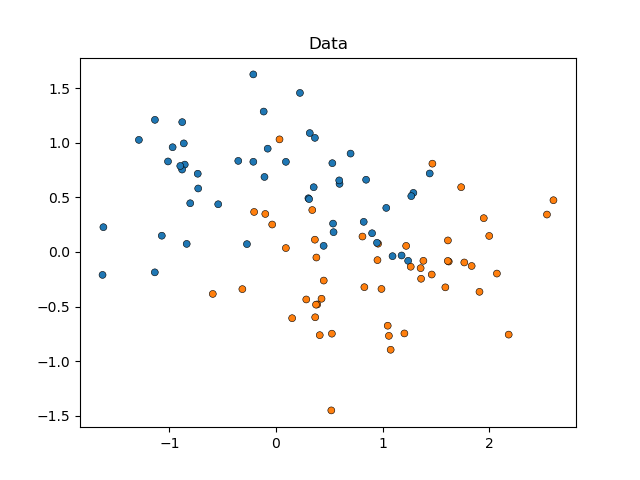
我們將從模擬月亮形狀的資料開始(其中類別之間的理想分隔是非線性的),並加入適度的雜訊。資料點將屬於兩個可能的類別之一,由兩個特徵來預測。我們將為每個類別模擬 50 個樣本
import matplotlib.pyplot as plt
import seaborn as sns

from sklearn.datasets import make_moons

X, y = make_moons(noise=0.352, random_state=1, n_samples=100)

sns.scatterplot(
    x=X[:, 0], y=X[:, 1], hue=y, marker="o", s=25, edgecolor="k", legend=False
).set_title("Data")
plt.show()
我們將比較 SVC 估算器在 kernel 參數上的效能,以決定此超參數的哪個選擇最能預測我們模擬的資料。我們將使用 RepeatedStratifiedKFold 評估模型的效能,重複 10 次 10 折分層交叉驗證,每次重複都使用不同的資料隨機化。效能將使用 roc_auc_score 進行評估。
from sklearn.model_selection import GridSearchCV, RepeatedStratifiedKFold
from sklearn.svm import SVC

param_grid = [
    {"kernel": ["linear"]},
    {"kernel": ["poly"], "degree": [2, 3]},
    {"kernel": ["rbf"]},
]

svc = SVC(random_state=0)

cv = RepeatedStratifiedKFold(n_splits=10, n_repeats=10, random_state=0)

search = GridSearchCV(estimator=svc, param_grid=param_grid, scoring="roc_auc", cv=cv)
search.fit(X, y)
我們現在可以檢查搜尋結果,並依其 mean_test_score 排序
import pandas as pd

results_df = pd.DataFrame(search.cv_results_)
results_df = results_df.sort_values(by=["rank_test_score"])
results_df = results_df.set_index(
    results_df["params"].apply(lambda x: "_".join(str(val) for val in x.values()))
).rename_axis("kernel")
results_df[["params", "rank_test_score", "mean_test_score", "std_test_score"]]
我們可以看到,使用 'rbf' 核的估算器表現最佳,緊隨其後的是 'linear'。使用 'poly' 核的兩個估算器表現較差,其中使用二度多項式的估算器效能比所有其他模型都低得多。
通常,分析到這裡就結束了,但遺漏了一半的故事。GridSearchCV 的輸出未提供有關模型之間差異確定性的資訊。我們不知道這些差異是否具有統計顯著性。為了評估這一點,我們需要進行統計檢定。具體而言,為了對比兩個模型的效能,我們應該統計比較其 AUC 分數。每個模型都有 100 個樣本(AUC 分數),因為我們重複了 10 次 10 折交叉驗證。
但是,模型的分數不是獨立的:所有模型都在相同的 100 個分割上進行評估,從而增加了模型效能之間的相關性。由於資料的某些分割可以使所有模型都特別容易或難以找到類別的區別,因此模型分數將會共變。
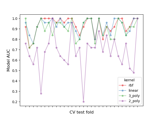
讓我們透過繪製每個折疊中所有模型的效能並計算折疊中模型之間的相關性來檢查此分割效應
# create df of model scores ordered by performance
model_scores = results_df.filter(regex=r"split\d*_test_score")

# plot 30 examples of dependency between cv fold and AUC scores
fig, ax = plt.subplots()
sns.lineplot(
    data=model_scores.transpose().iloc[:30],
    dashes=False,
    palette="Set1",
    marker="o",
    alpha=0.5,
    ax=ax,
)
ax.set_xlabel("CV test fold", size=12, labelpad=10)
ax.set_ylabel("Model AUC", size=12)
ax.tick_params(bottom=True, labelbottom=False)
plt.show()

# print correlation of AUC scores across folds
print(f"Correlation of models:\n {model_scores.transpose().corr()}")
Correlation of models:
 kernel       rbf    linear    3_poly    2_poly
kernel
rbf     1.000000  0.882561  0.783392  0.351390
linear  0.882561  1.000000  0.746492  0.298688
3_poly  0.783392  0.746492  1.000000  0.355440
2_poly  0.351390  0.298688  0.355440  1.000000
我們可以觀察到模型的效能高度取決於折疊。
因此,如果我們假設樣本之間存在獨立性,我們將低估統計檢定中計算的變異數,從而增加假陽性錯誤的數量(即,在模型之間不存在顯著差異時檢測到顯著差異) [1]。
針對這些情況開發了幾種變異數校正統計檢定。在此範例中,我們將展示如何在兩種不同的統計框架下實作其中一種檢定(所謂的 Nadeau 和 Bengio 校正 t 檢定):頻率論和貝氏。
比較兩個模型:頻率論方法#
我們可以從問:「當按 mean_test_score 排名時,第一個模型是否明顯優於第二個模型?」開始
為了使用頻率論方法回答這個問題,我們可以執行成對 t 檢定並計算 p 值。這在預測文獻中也稱為 Diebold-Mariano 檢定 [5]。已經開發了這種 t 檢定的許多變體,以解決上一節中描述的「樣本非獨立性問題」。我們將使用經證明可獲得最高可重複性分數(評估模型在評估同一資料集的不同隨機分割時的效能有多相似)同時保持低假陽性和假陰性率的分數:Nadeau 和 Bengio 的校正 t 檢定 [2],該檢定使用 10 次重複的 10 折交叉驗證 [3]。
此校正的成對 t 檢定計算如下
其中,\(k\) 是折數,\(r\) 是交叉驗證中的重複次數,\(x\) 是模型效能的差異,\(n_{test}\) 是用於測試的樣本數,\(n_{train}\) 是用於訓練的樣本數,而 \(\hat{\sigma}^2\) 代表觀察到的差異的變異數。
讓我們實作一個修正後的右尾配對 t 檢定,以評估第一個模型的效能是否顯著優於第二個模型。我們的虛無假設是第二個模型的效能至少與第一個模型一樣好。
import numpy as np
from scipy.stats import t


def corrected_std(differences, n_train, n_test):
    """Corrects standard deviation using Nadeau and Bengio's approach.

    Parameters
    ----------
    differences : ndarray of shape (n_samples,)
        Vector containing the differences in the score metrics of two models.
    n_train : int
        Number of samples in the training set.
    n_test : int
        Number of samples in the testing set.

    Returns
    -------
    corrected_std : float
        Variance-corrected standard deviation of the set of differences.
    """
    # kr = k times r, r times repeated k-fold crossvalidation,
    # kr equals the number of times the model was evaluated
    kr = len(differences)
    corrected_var = np.var(differences, ddof=1) * (1 / kr + n_test / n_train)
    corrected_std = np.sqrt(corrected_var)
    return corrected_std


def compute_corrected_ttest(differences, df, n_train, n_test):
    """Computes right-tailed paired t-test with corrected variance.

    Parameters
    ----------
    differences : array-like of shape (n_samples,)
        Vector containing the differences in the score metrics of two models.
    df : int
        Degrees of freedom.
    n_train : int
        Number of samples in the training set.
    n_test : int
        Number of samples in the testing set.

    Returns
    -------
    t_stat : float
        Variance-corrected t-statistic.
    p_val : float
        Variance-corrected p-value.
    """
    mean = np.mean(differences)
    std = corrected_std(differences, n_train, n_test)
    t_stat = mean / std
    p_val = t.sf(np.abs(t_stat), df)  # right-tailed t-test
    return t_stat, p_val
model_1_scores = model_scores.iloc[0].values  # scores of the best model
model_2_scores = model_scores.iloc[1].values  # scores of the second-best model

differences = model_1_scores - model_2_scores

n = differences.shape[0]  # number of test sets
df = n - 1
n_train = len(list(cv.split(X, y))[0][0])
n_test = len(list(cv.split(X, y))[0][1])

t_stat, p_val = compute_corrected_ttest(differences, df, n_train, n_test)
print(f"Corrected t-value: {t_stat:.3f}\nCorrected p-value: {p_val:.3f}")
Corrected t-value: 0.750
Corrected p-value: 0.227
我們可以將修正後的 t 值和 p 值與未修正的值進行比較。
Uncorrected t-value: 2.611
Uncorrected p-value: 0.005
使用傳統的顯著性 alpha 水準 p=0.05,我們觀察到未修正的 t 檢定結論是第一個模型顯著優於第二個模型。
相反地,使用修正的方法,我們無法檢測到這種差異。
然而,在後者情況下,頻率論方法不允許我們得出第一個和第二個模型的效能相當的結論。如果我們想做出這種斷言,我們需要使用貝氏方法。
比較兩個模型:貝氏方法#
我們可以利用貝氏估計來計算第一個模型優於第二個模型的機率。貝氏估計將輸出一個分佈,接著是兩個模型效能差異的平均值 \(\mu\)。
為了獲得後驗分佈,我們需要定義一個先驗,在觀察資料之前對平均值的分配情況進行建模,並將其乘以一個可能性函數,該函數計算在平均值可能採用的情況下,我們觀察到的差異有多大的可能性。
貝氏估計可以以多種形式進行以回答我們的問題,但在這個例子中,我們將實作 Benavoli 及其同事建議的方法 [4]。
使用封閉形式表示式定義我們的後驗的一種方法是選擇與可能性函數共軛的先驗。Benavoli 及其同事 [4] 表明,當比較兩個分類器的效能時,我們可以將先驗建模為 Normal-Gamma 分佈(平均值和變異數均未知),該分佈與常態可能性共軛,從而將後驗表示為常態分佈。從這個常態後驗中邊際化變異數,我們可以將平均參數的後驗定義為 Student's t 分佈。具體來說
其中,\(n\) 是樣本總數,\(\overline{x}\) 代表分數的平均差異,\(n_{test}\) 是用於測試的樣本數,\(n_{train}\) 是用於訓練的樣本數,而 \(\hat{\sigma}^2\) 代表觀察到的差異的變異數。
請注意,我們在貝氏方法中也使用了 Nadeau 和 Bengio 的修正變異數。
讓我們計算並繪製後驗。
讓我們繪製後驗分佈。
x = np.linspace(t_post.ppf(0.001), t_post.ppf(0.999), 100)

plt.plot(x, t_post.pdf(x))
plt.xticks(np.arange(-0.04, 0.06, 0.01))
plt.fill_between(x, t_post.pdf(x), 0, facecolor="blue", alpha=0.2)
plt.ylabel("Probability density")
plt.xlabel(r"Mean difference ($\mu$)")
plt.title("Posterior distribution")
plt.show()
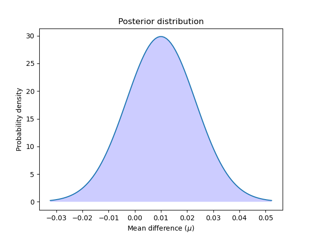
我們可以透過計算從零到無限大的後驗分佈曲線下的面積來計算第一個模型優於第二個模型的機率。反之亦然:我們可以透過計算從負無限大到零的曲線下的面積來計算第二個模型優於第一個模型的機率。
better_prob = 1 - t_post.cdf(0)

print(
    f"Probability of {model_scores.index[0]} being more accurate than "
    f"{model_scores.index[1]}: {better_prob:.3f}"
)
print(
    f"Probability of {model_scores.index[1]} being more accurate than "
    f"{model_scores.index[0]}: {1 - better_prob:.3f}"
)
Probability of rbf being more accurate than linear: 0.773
Probability of linear being more accurate than rbf: 0.227
與頻率論方法相反,我們可以計算一個模型優於另一個模型的機率。
請注意,我們獲得了與頻率論方法相似的結果。鑑於我們選擇的先驗,我們本質上執行相同的計算,但我們被允許做出不同的斷言。
實質等效區域#
有時,我們有興趣確定我們的模型具有相等效能的機率,其中「相等」是以實際的方式定義的。一種簡單的方法 [4] 是將估計器的準確度差異小於 1% 時定義為實際上相等。但是我們也可以考慮我們試圖解決的問題來定義這種實際等效性。例如,準確度相差 5% 將意味著銷售額增加 1000 美元,我們認為任何高於該數量的數量都與我們的業務相關。
在這個範例中,我們將實質等效區域 (ROPE) 定義為 \([-0.01, 0.01]\)。也就是說,如果兩個模型在效能上的差異小於 1%,我們將認為它們實際上是相等的。
為了計算分類器實際上相等的機率,我們計算 ROPE 間隔上後驗曲線下的面積。
rope_interval = [-0.01, 0.01]
rope_prob = t_post.cdf(rope_interval[1]) - t_post.cdf(rope_interval[0])

print(
    f"Probability of {model_scores.index[0]} and {model_scores.index[1]} "
    f"being practically equivalent: {rope_prob:.3f}"
)
Probability of rbf and linear being practically equivalent: 0.432
我們可以繪製後驗在 ROPE 間隔上的分佈情況。
x_rope = np.linspace(rope_interval[0], rope_interval[1], 100)

plt.plot(x, t_post.pdf(x))
plt.xticks(np.arange(-0.04, 0.06, 0.01))
plt.vlines([-0.01, 0.01], ymin=0, ymax=(np.max(t_post.pdf(x)) + 1))
plt.fill_between(x_rope, t_post.pdf(x_rope), 0, facecolor="blue", alpha=0.2)
plt.ylabel("Probability density")
plt.xlabel(r"Mean difference ($\mu$)")
plt.title("Posterior distribution under the ROPE")
plt.show()
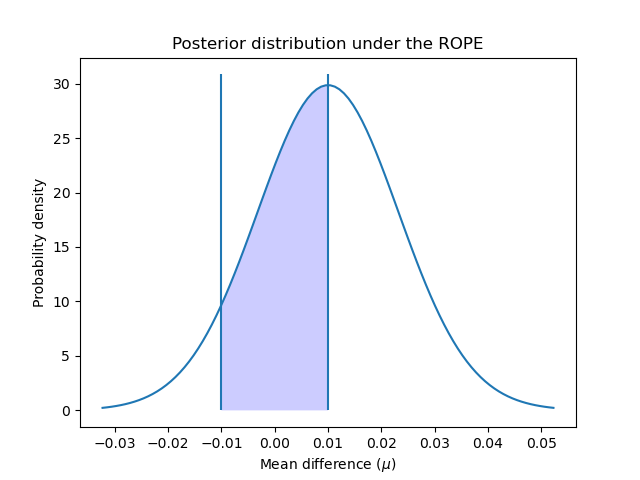
如 [4] 中建議,我們可以進一步使用與頻率論方法相同的標準來解釋這些機率:落在 ROPE 內的機率是否大於 95%(alpha 值為 5%)?在這種情況下,我們可以得出結論,兩個模型實際上是相等的。
貝氏估計方法還允許我們計算我們對差異估計的不確定性。這可以使用可信區間來計算。對於給定的機率,它們顯示了估計量(在我們的例子中是效能的平均差異)可以採用的值範圍。例如,50% 的可信區間 [x, y] 告訴我們,模型之間效能的真實(平均)差異有 50% 的機率介於 x 和 y 之間。
讓我們使用 50%、75% 和 95% 來確定我們資料的可信區間。
cred_intervals = []
intervals = [0.5, 0.75, 0.95]

for interval in intervals:
    cred_interval = list(t_post.interval(interval))
    cred_intervals.append([interval, cred_interval[0], cred_interval[1]])

cred_int_df = pd.DataFrame(
    cred_intervals, columns=["interval", "lower value", "upper value"]
).set_index("interval")
cred_int_df
如表格所示,模型之間的真實平均差異有 50% 的機率介於 0.000977 和 0.019023 之間,有 70% 的機率介於 -0.005422 和 0.025422 之間,有 95% 的機率介於 -0.016445 和 0.036445 之間。
所有模型的成對比較:頻率論方法#
我們可能也有興趣比較使用 GridSearchCV 評估的所有模型的效能。在這種情況下,我們將多次執行我們的統計測試,這將導致 多重比較問題。
有很多可能的方法來解決這個問題,但標準方法是應用 Bonferroni 校正。Bonferroni 可以透過將 p 值乘以我們要測試的比較次數來計算。
讓我們使用修正後的 t 檢定比較模型的效能。
from itertools import combinations
from math import factorial

n_comparisons = factorial(len(model_scores)) / (
    factorial(2) * factorial(len(model_scores) - 2)
)
pairwise_t_test = []

for model_i, model_k in combinations(range(len(model_scores)), 2):
    model_i_scores = model_scores.iloc[model_i].values
    model_k_scores = model_scores.iloc[model_k].values
    differences = model_i_scores - model_k_scores
    t_stat, p_val = compute_corrected_ttest(differences, df, n_train, n_test)
    p_val *= n_comparisons  # implement Bonferroni correction
    # Bonferroni can output p-values higher than 1
    p_val = 1 if p_val > 1 else p_val
    pairwise_t_test.append(
        [model_scores.index[model_i], model_scores.index[model_k], t_stat, p_val]
    )

pairwise_comp_df = pd.DataFrame(
    pairwise_t_test, columns=["model_1", "model_2", "t_stat", "p_val"]
).round(3)
pairwise_comp_df
我們觀察到,在修正多重比較後,唯一與其他模型顯著不同的模型是 '2_poly'。 GridSearchCV 排名第一的模型 'rbf' 與 'linear' 或 '3_poly' 沒有顯著差異。
所有模型的成對比較:貝氏方法#
當使用貝氏估計來比較多個模型時,我們不需要修正多重比較(關於原因請參閱 [4])。
我們可以以第一節相同的方式執行我們的成對比較。
pairwise_bayesian = []

for model_i, model_k in combinations(range(len(model_scores)), 2):
    model_i_scores = model_scores.iloc[model_i].values
    model_k_scores = model_scores.iloc[model_k].values
    differences = model_i_scores - model_k_scores
    t_post = t(
        df, loc=np.mean(differences), scale=corrected_std(differences, n_train, n_test)
    )
    worse_prob = t_post.cdf(rope_interval[0])
    better_prob = 1 - t_post.cdf(rope_interval[1])
    rope_prob = t_post.cdf(rope_interval[1]) - t_post.cdf(rope_interval[0])

    pairwise_bayesian.append([worse_prob, better_prob, rope_prob])

pairwise_bayesian_df = pd.DataFrame(
    pairwise_bayesian, columns=["worse_prob", "better_prob", "rope_prob"]
).round(3)

pairwise_comp_df = pairwise_comp_df.join(pairwise_bayesian_df)
pairwise_comp_df
使用貝氏方法,我們可以計算一個模型的效能優於、劣於或實際上等於另一個模型的機率。
結果顯示,GridSearchCV 排名第一的模型 'rbf',有大約 6.8% 的機率劣於 'linear',以及 1.8% 的機率劣於 '3_poly'。'rbf' 和 'linear' 有 43% 的機率實際上是相等的,而 'rbf' 和 '3_poly' 有 10% 的機率是相等的。
與使用頻率論方法獲得的結論類似,所有模型都有 100% 的機率優於 '2_poly',並且沒有任何模型的效能與後者實際上相等。
重點訊息#
效能測量中的微小差異可能很容易被證明僅僅是偶然的,而不是因為一個模型系統性地預測得比另一個好。如本例所示,統計可以告訴您這種可能性有多大。
當統計上比較在 GridSearchCV 中評估的兩個模型的效能時,必須修正計算出的變異數,因為模型的得分彼此之間不是獨立的,因此可能被低估。
使用(變異數修正的)配對 t 檢定的頻率論方法可以告訴我們一個模型的效能是否優於另一個模型,並且確定程度高於偶然。
貝氏方法可以提供一個模型優於、劣於或實際上等於另一個模型的機率。它還可以告訴我們,我們有多大把握知道我們模型的真實差異落在某個值範圍內。
如果對多個模型進行統計比較,則在使用頻率論方法時需要進行多重比較校正。
參考文獻
腳本總執行時間: (0 分鐘 1.644 秒)
相關範例