使用多任務 Lasso 進行聯合特徵選擇#

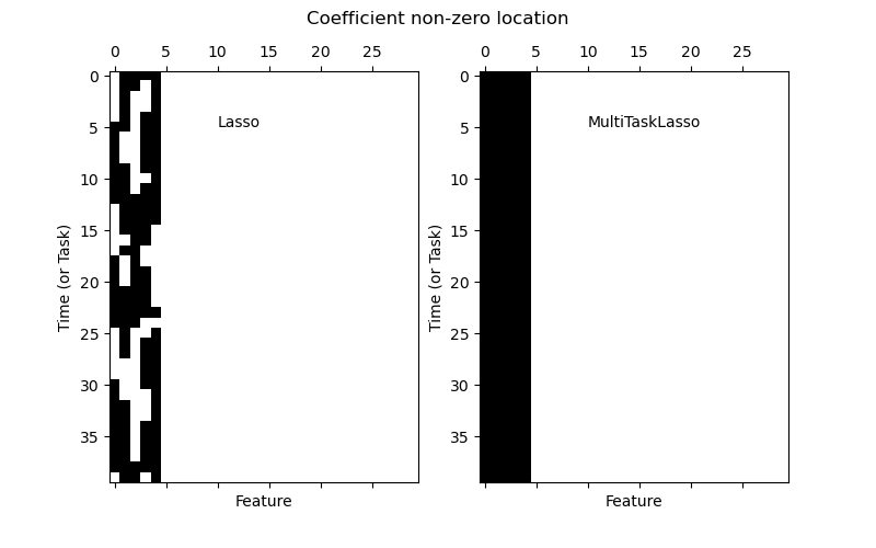
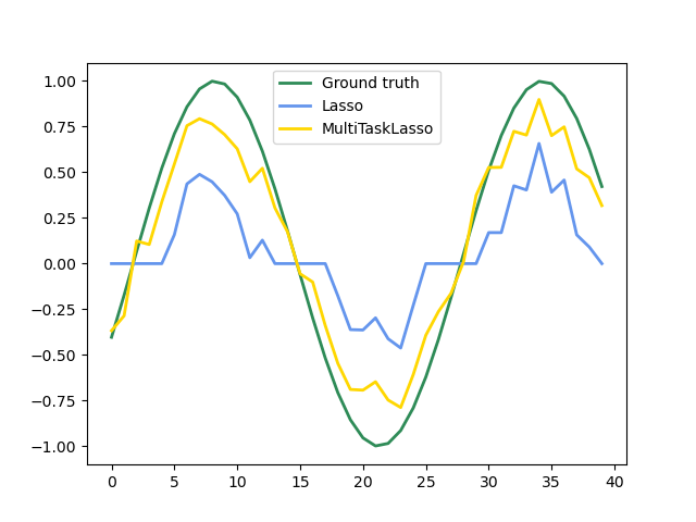
多任務 lasso 允許聯合擬合多個迴歸問題，強制在任務之間選擇相同的特徵。此範例模擬循序量測，每個任務都是一個時間點，相關特徵的振幅隨時間變化，但保持不變。多任務 lasso 強制在一個時間點選取的特徵在所有時間點都被選取。這使得 Lasso 的特徵選擇更穩定。

# Authors: The scikit-learn developers
# SPDX-License-Identifier: BSD-3-Clause

產生資料#

import numpy as np

rng = np.random.RandomState(42)

# Generate some 2D coefficients with sine waves with random frequency and phase
n_samples, n_features, n_tasks = 100, 30, 40
n_relevant_features = 5
coef = np.zeros((n_tasks, n_features))
times = np.linspace(0, 2 * np.pi, n_tasks)
for k in range(n_relevant_features):
    coef[:, k] = np.sin((1.0 + rng.randn(1)) * times + 3 * rng.randn(1))

X = rng.randn(n_samples, n_features)
Y = np.dot(X, coef.T) + rng.randn(n_samples, n_tasks)

擬合模型#

from sklearn.linear_model import Lasso, MultiTaskLasso

coef_lasso_ = np.array([Lasso(alpha=0.5).fit(X, y).coef_ for y in Y.T])
coef_multi_task_lasso_ = MultiTaskLasso(alpha=1.0).fit(X, Y).coef_

繪製支持和時間序列#

import matplotlib.pyplot as plt

fig = plt.figure(figsize=(8, 5))
plt.subplot(1, 2, 1)
plt.spy(coef_lasso_)
plt.xlabel("Feature")
plt.ylabel("Time (or Task)")
plt.text(10, 5, "Lasso")
plt.subplot(1, 2, 2)
plt.spy(coef_multi_task_lasso_)
plt.xlabel("Feature")
plt.ylabel("Time (or Task)")
plt.text(10, 5, "MultiTaskLasso")
fig.suptitle("Coefficient non-zero location")

feature_to_plot = 0
plt.figure()
lw = 2
plt.plot(coef[:, feature_to_plot], color="seagreen", linewidth=lw, label="Ground truth")
plt.plot(
    coef_lasso_[:, feature_to_plot], color="cornflowerblue", linewidth=lw, label="Lasso"
)
plt.plot(
    coef_multi_task_lasso_[:, feature_to_plot],
    color="gold",
    linewidth=lw,
    label="MultiTaskLasso",
)
plt.legend(loc="upper center")
plt.axis("tight")
plt.ylim([-1.1, 1.1])
plt.show()