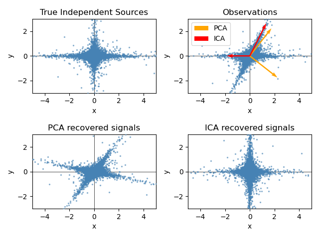
2D 點雲上的 FastICA#

此範例在特徵空間中視覺化地說明了使用兩種不同成分分析技術的結果比較。

在特徵空間中表示 ICA 可以顯示「幾何 ICA」：ICA 是一種在特徵空間中尋找方向的演算法，這些方向對應於具有高非高斯性的投影。這些方向在原始特徵空間中不必正交，但在白化特徵空間中是正交的，在白化特徵空間中，所有方向都對應於相同的變異數。

另一方面，PCA 在原始特徵空間中尋找正交方向，這些方向對應於解釋最大變異數的方向。

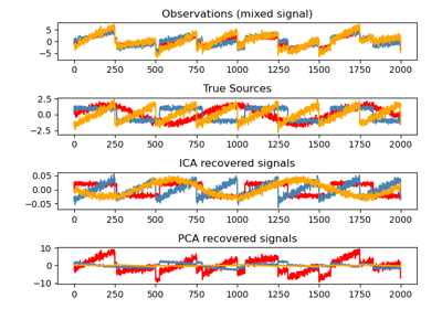
在這裡，我們使用高度非高斯過程 (2 個具有低自由度的學生 T，左上圖) 模擬獨立來源。我們將它們混合以建立觀測 (右上圖)。在這個原始觀測空間中，由 PCA 識別的方向由橙色向量表示。我們在 PCA 空間中表示訊號，在依據對應於 PCA 向量的變異數進行白化後 (左下)。執行 ICA 對應於在此空間中尋找旋轉，以識別最大非高斯性的方向 (右下)。

# Authors: The scikit-learn developers
# SPDX-License-Identifier: BSD-3-Clause

產生樣本資料#

import numpy as np

from sklearn.decomposition import PCA, FastICA

rng = np.random.RandomState(42)
S = rng.standard_t(1.5, size=(20000, 2))
S[:, 0] *= 2.0

# Mix data
A = np.array([[1, 1], [0, 2]])  # Mixing matrix

X = np.dot(S, A.T)  # Generate observations

pca = PCA()
S_pca_ = pca.fit(X).transform(X)

ica = FastICA(random_state=rng, whiten="arbitrary-variance")
S_ica_ = ica.fit(X).transform(X)  # Estimate the sources

繪製結果圖#

import matplotlib.pyplot as plt


def plot_samples(S, axis_list=None):
    plt.scatter(
        S[:, 0], S[:, 1], s=2, marker="o", zorder=10, color="steelblue", alpha=0.5
    )
    if axis_list is not None:
        for axis, color, label in axis_list:
            x_axis, y_axis = axis / axis.std()
            plt.quiver(
                (0, 0),
                (0, 0),
                x_axis,
                y_axis,
                zorder=11,
                width=0.01,
                scale=6,
                color=color,
                label=label,
            )

    plt.hlines(0, -5, 5, color="black", linewidth=0.5)
    plt.vlines(0, -3, 3, color="black", linewidth=0.5)
    plt.xlim(-5, 5)
    plt.ylim(-3, 3)
    plt.gca().set_aspect("equal")
    plt.xlabel("x")
    plt.ylabel("y")


plt.figure()
plt.subplot(2, 2, 1)
plot_samples(S / S.std())
plt.title("True Independent Sources")

axis_list = [(pca.components_.T, "orange", "PCA"), (ica.mixing_, "red", "ICA")]
plt.subplot(2, 2, 2)
plot_samples(X / np.std(X), axis_list=axis_list)
legend = plt.legend(loc="upper left")
legend.set_zorder(100)

plt.title("Observations")

plt.subplot(2, 2, 3)
plot_samples(S_pca_ / np.std(S_pca_))
plt.title("PCA recovered signals")

plt.subplot(2, 2, 4)
plot_samples(S_ica_ / np.std(S_ica_))
plt.title("ICA recovered signals")

plt.subplots_adjust(0.09, 0.04, 0.94, 0.94, 0.26, 0.36)
plt.tight_layout()
plt.show()