轉換回歸模型目標的影響#

在本範例中，我們概述了 TransformedTargetRegressor。我們使用兩個範例來說明在學習線性回歸模型之前轉換目標的好處。第一個範例使用合成資料，而第二個範例則基於 Ames 房屋資料集。

# Authors: The scikit-learn developers
# SPDX-License-Identifier: BSD-3-Clause

print(__doc__)

合成範例#

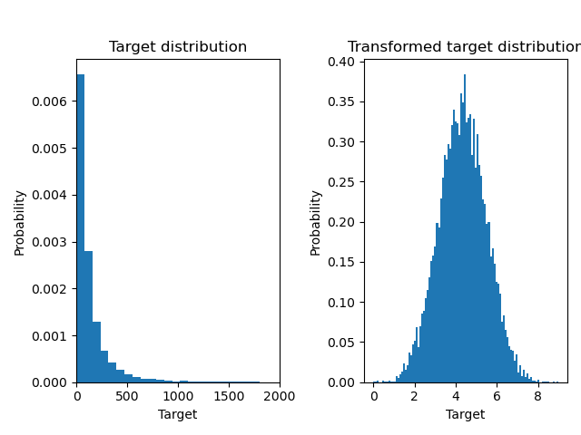
產生合成的隨機回歸資料集。目標 y 被修改為

平移所有目標，使所有條目均為非負數（透過加入最低 y 的絕對值），以及
應用指數函數以取得無法使用簡單線性模型擬合的非線性目標。

因此，將在訓練線性回歸模型並用於預測之前，使用對數 (np.log1p) 和指數函數 (np.expm1) 來轉換目標。

import numpy as np

from sklearn.datasets import make_regression

X, y = make_regression(n_samples=10_000, noise=100, random_state=0)
y = np.expm1((y + abs(y.min())) / 200)
y_trans = np.log1p(y)

下面我們繪製了在應用對數函數之前和之後的目標機率密度函數。

import matplotlib.pyplot as plt

from sklearn.model_selection import train_test_split

f, (ax0, ax1) = plt.subplots(1, 2)

ax0.hist(y, bins=100, density=True)
ax0.set_xlim([0, 2000])
ax0.set_ylabel("Probability")
ax0.set_xlabel("Target")
ax0.set_title("Target distribution")

ax1.hist(y_trans, bins=100, density=True)
ax1.set_ylabel("Probability")
ax1.set_xlabel("Target")
ax1.set_title("Transformed target distribution")

f.suptitle("Synthetic data", y=1.05)
plt.tight_layout()

X_train, X_test, y_train, y_test = train_test_split(X, y, random_state=0)

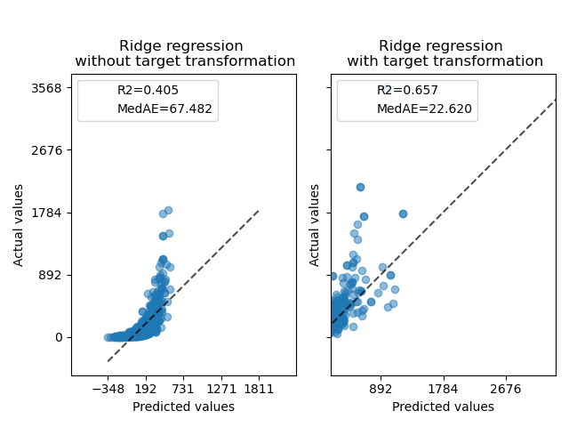
Synthetic data, Target distribution, Transformed target distribution

首先，將在原始目標上應用線性模型。由於非線性，訓練後的模型在預測期間將不精確。隨後，使用對數函數來線性化目標，即使使用類似的線性模型，也能獲得更好的預測，如中位數絕對誤差 (MedAE) 所報告的那樣。

from sklearn.metrics import median_absolute_error, r2_score


def compute_score(y_true, y_pred):
    return {
        "R2": f"{r2_score(y_true, y_pred):.3f}",
        "MedAE": f"{median_absolute_error(y_true, y_pred):.3f}",
    }

from sklearn.compose import TransformedTargetRegressor
from sklearn.linear_model import RidgeCV
from sklearn.metrics import PredictionErrorDisplay

f, (ax0, ax1) = plt.subplots(1, 2, sharey=True)

ridge_cv = RidgeCV().fit(X_train, y_train)
y_pred_ridge = ridge_cv.predict(X_test)

ridge_cv_with_trans_target = TransformedTargetRegressor(
    regressor=RidgeCV(), func=np.log1p, inverse_func=np.expm1
).fit(X_train, y_train)
y_pred_ridge_with_trans_target = ridge_cv_with_trans_target.predict(X_test)

PredictionErrorDisplay.from_predictions(
    y_test,
    y_pred_ridge,
    kind="actual_vs_predicted",
    ax=ax0,
    scatter_kwargs={"alpha": 0.5},
)
PredictionErrorDisplay.from_predictions(
    y_test,
    y_pred_ridge_with_trans_target,
    kind="actual_vs_predicted",
    ax=ax1,
    scatter_kwargs={"alpha": 0.5},
)

# Add the score in the legend of each axis
for ax, y_pred in zip([ax0, ax1], [y_pred_ridge, y_pred_ridge_with_trans_target]):
    for name, score in compute_score(y_test, y_pred).items():
        ax.plot([], [], " ", label=f"{name}={score}")
    ax.legend(loc="upper left")

ax0.set_title("Ridge regression \n without target transformation")
ax1.set_title("Ridge regression \n with target transformation")
f.suptitle("Synthetic data", y=1.05)
plt.tight_layout()

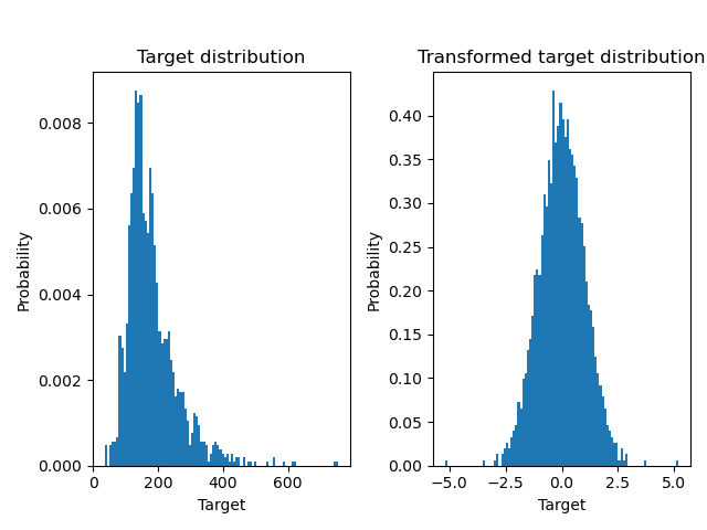
Synthetic data, Ridge regression without target transformation, Ridge regression with target transformation

真實世界資料集#

以類似的方式，使用 Ames 房屋資料集來說明在學習模型之前轉換目標的影響。在本範例中，要預測的目標是每棟房屋的售價。

from sklearn.datasets import fetch_openml
from sklearn.preprocessing import quantile_transform

ames = fetch_openml(name="house_prices", as_frame=True)
# Keep only numeric columns
X = ames.data.select_dtypes(np.number)
# Remove columns with NaN or Inf values
X = X.drop(columns=["LotFrontage", "GarageYrBlt", "MasVnrArea"])
# Let the price be in k$
y = ames.target / 1000
y_trans = quantile_transform(
    y.to_frame(), n_quantiles=900, output_distribution="normal", copy=True
).squeeze()

使用 QuantileTransformer 在應用 RidgeCV 模型之前正規化目標分佈。

f, (ax0, ax1) = plt.subplots(1, 2)

ax0.hist(y, bins=100, density=True)
ax0.set_ylabel("Probability")
ax0.set_xlabel("Target")
ax0.set_title("Target distribution")

ax1.hist(y_trans, bins=100, density=True)
ax1.set_ylabel("Probability")
ax1.set_xlabel("Target")
ax1.set_title("Transformed target distribution")

f.suptitle("Ames housing data: selling price", y=1.05)
plt.tight_layout()

Ames housing data: selling price, Target distribution, Transformed target distribution

X_train, X_test, y_train, y_test = train_test_split(X, y, random_state=1)

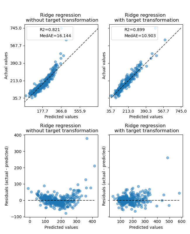
轉換器的效果弱於合成資料。但是，轉換會導致 \(R^2\) 增加，並且 MedAE 大幅減少。沒有目標轉換的殘差圖（預測目標 - 真實目標 vs. 預測目標）由於殘差值因預測目標值而異，因此呈現彎曲的「反向微笑」形狀。使用目標轉換時，形狀更線性，表示模型擬合更好。

from sklearn.preprocessing import QuantileTransformer

f, (ax0, ax1) = plt.subplots(2, 2, sharey="row", figsize=(6.5, 8))

ridge_cv = RidgeCV().fit(X_train, y_train)
y_pred_ridge = ridge_cv.predict(X_test)

ridge_cv_with_trans_target = TransformedTargetRegressor(
    regressor=RidgeCV(),
    transformer=QuantileTransformer(n_quantiles=900, output_distribution="normal"),
).fit(X_train, y_train)
y_pred_ridge_with_trans_target = ridge_cv_with_trans_target.predict(X_test)

# plot the actual vs predicted values
PredictionErrorDisplay.from_predictions(
    y_test,
    y_pred_ridge,
    kind="actual_vs_predicted",
    ax=ax0[0],
    scatter_kwargs={"alpha": 0.5},
)
PredictionErrorDisplay.from_predictions(
    y_test,
    y_pred_ridge_with_trans_target,
    kind="actual_vs_predicted",
    ax=ax0[1],
    scatter_kwargs={"alpha": 0.5},
)

# Add the score in the legend of each axis
for ax, y_pred in zip([ax0[0], ax0[1]], [y_pred_ridge, y_pred_ridge_with_trans_target]):
    for name, score in compute_score(y_test, y_pred).items():
        ax.plot([], [], " ", label=f"{name}={score}")
    ax.legend(loc="upper left")

ax0[0].set_title("Ridge regression \n without target transformation")
ax0[1].set_title("Ridge regression \n with target transformation")

# plot the residuals vs the predicted values
PredictionErrorDisplay.from_predictions(
    y_test,
    y_pred_ridge,
    kind="residual_vs_predicted",
    ax=ax1[0],
    scatter_kwargs={"alpha": 0.5},
)
PredictionErrorDisplay.from_predictions(
    y_test,
    y_pred_ridge_with_trans_target,
    kind="residual_vs_predicted",
    ax=ax1[1],
    scatter_kwargs={"alpha": 0.5},
)
ax1[0].set_title("Ridge regression \n without target transformation")
ax1[1].set_title("Ridge regression \n with target transformation")

f.suptitle("Ames housing data: selling price", y=1.05)
plt.tight_layout()
plt.show()