使用多項式邏輯迴歸 + L1 的 MNIST 分類#

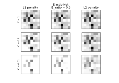
在這裡，我們在 MNIST 數字分類任務的子集上擬合具有 L1 懲罰的多項式邏輯迴歸。我們為此目的使用 SAGA 演算法：當樣本數量明顯大於特徵數量時，此求解器速度很快，並且能夠精細地優化非平滑目標函數，而這正是 l1 懲罰的情況。測試準確度達到 > 0.8，而權重向量保持稀疏，因此更容易解釋。

請注意，此 l1 懲罰的線性模型的準確度明顯低於在此資料集上使用 l2 懲罰的線性模型或非線性多層感知器模型所能達到的準確度。

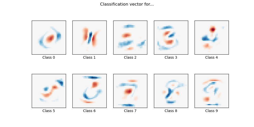
Sparsity with L1 penalty: 74.57%
Test score with L1 penalty: 0.8253
Example run in 8.308 s

# Authors: The scikit-learn developers
# SPDX-License-Identifier: BSD-3-Clause

import time

import matplotlib.pyplot as plt
import numpy as np

from sklearn.datasets import fetch_openml
from sklearn.linear_model import LogisticRegression
from sklearn.model_selection import train_test_split
from sklearn.preprocessing import StandardScaler
from sklearn.utils import check_random_state

# Turn down for faster convergence
t0 = time.time()
train_samples = 5000

# Load data from https://www.openml.org/d/554
X, y = fetch_openml("mnist_784", version=1, return_X_y=True, as_frame=False)

random_state = check_random_state(0)
permutation = random_state.permutation(X.shape[0])
X = X[permutation]
y = y[permutation]
X = X.reshape((X.shape[0], -1))

X_train, X_test, y_train, y_test = train_test_split(
    X, y, train_size=train_samples, test_size=10000
)

scaler = StandardScaler()
X_train = scaler.fit_transform(X_train)
X_test = scaler.transform(X_test)

# Turn up tolerance for faster convergence
clf = LogisticRegression(C=50.0 / train_samples, penalty="l1", solver="saga", tol=0.1)
clf.fit(X_train, y_train)
sparsity = np.mean(clf.coef_ == 0) * 100
score = clf.score(X_test, y_test)
# print('Best C % .4f' % clf.C_)
print("Sparsity with L1 penalty: %.2f%%" % sparsity)
print("Test score with L1 penalty: %.4f" % score)

coef = clf.coef_.copy()
plt.figure(figsize=(10, 5))
scale = np.abs(coef).max()
for i in range(10):
    l1_plot = plt.subplot(2, 5, i + 1)
    l1_plot.imshow(
        coef[i].reshape(28, 28),
        interpolation="nearest",
        cmap=plt.cm.RdBu,
        vmin=-scale,
        vmax=scale,
    )
    l1_plot.set_xticks(())
    l1_plot.set_yticks(())
    l1_plot.set_xlabel("Class %i" % i)
plt.suptitle("Classification vector for...")

run_time = time.time() - t0
print("Example run in %.3f s" % run_time)
plt.show()