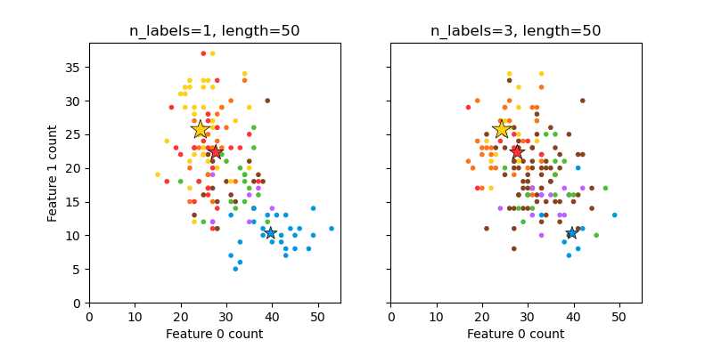
繪製隨機產生的多標籤資料集#

這說明了 make_multilabel_classification 資料集產生器。每個樣本由兩個特徵的計數組成（總共最多 50 個），這些特徵在兩個類別中的分布不同。

點的標記方式如下，其中 Y 表示該類別存在

1	2	3	顏色
Y	N	N	紅色
N	Y	N	藍色
N	N	Y	黃色
Y	Y	N	紫色
Y	N	Y	橙色
Y	Y	N	綠色
Y	Y	Y	棕色

星號標記每個類別的預期樣本；其大小反映選擇該類別標籤的機率。

左側和右側範例突顯了 n_labels 參數：右側圖中的更多樣本有 2 或 3 個標籤。

請注意，這個二維範例非常退化：通常特徵的數量會遠大於「文件長度」，而這裡我們的文件比詞彙量大得多。同樣地，當 n_classes > n_features 時，特徵區分特定類別的可能性會小得多。

n_labels=1, length=50, n_labels=3, length=50

The data was generated from (random_state=521):
Class   P(C)    P(w0|C) P(w1|C)
red     0.32    0.55    0.45
blue    0.26    0.79    0.21
yellow  0.42    0.49    0.51

# Authors: The scikit-learn developers
# SPDX-License-Identifier: BSD-3-Clause

import matplotlib.pyplot as plt
import numpy as np

from sklearn.datasets import make_multilabel_classification as make_ml_clf

COLORS = np.array(
    [
        "!",
        "#FF3333",  # red
        "#0198E1",  # blue
        "#BF5FFF",  # purple
        "#FCD116",  # yellow
        "#FF7216",  # orange
        "#4DBD33",  # green
        "#87421F",  # brown
    ]
)

# Use same random seed for multiple calls to make_multilabel_classification to
# ensure same distributions
RANDOM_SEED = np.random.randint(2**10)


def plot_2d(ax, n_labels=1, n_classes=3, length=50):
    X, Y, p_c, p_w_c = make_ml_clf(
        n_samples=150,
        n_features=2,
        n_classes=n_classes,
        n_labels=n_labels,
        length=length,
        allow_unlabeled=False,
        return_distributions=True,
        random_state=RANDOM_SEED,
    )

    ax.scatter(
        X[:, 0], X[:, 1], color=COLORS.take((Y * [1, 2, 4]).sum(axis=1)), marker="."
    )
    ax.scatter(
        p_w_c[0] * length,
        p_w_c[1] * length,
        marker="*",
        linewidth=0.5,
        edgecolor="black",
        s=20 + 1500 * p_c**2,
        color=COLORS.take([1, 2, 4]),
    )
    ax.set_xlabel("Feature 0 count")
    return p_c, p_w_c


_, (ax1, ax2) = plt.subplots(1, 2, sharex="row", sharey="row", figsize=(8, 4))
plt.subplots_adjust(bottom=0.15)

p_c, p_w_c = plot_2d(ax1, n_labels=1)
ax1.set_title("n_labels=1, length=50")
ax1.set_ylabel("Feature 1 count")

plot_2d(ax2, n_labels=3)
ax2.set_title("n_labels=3, length=50")
ax2.set_xlim(left=0, auto=True)
ax2.set_ylim(bottom=0, auto=True)

plt.show()

print("The data was generated from (random_state=%d):" % RANDOM_SEED)
print("Class", "P(C)", "P(w0|C)", "P(w1|C)", sep="\t")
for k, p, p_w in zip(["red", "blue", "yellow"], p_c, p_w_c.T):
    print("%s\t%0.2f\t%0.2f\t%0.2f" % (k, p, p_w[0], p_w[1]))