在斷裂球體上的流形學習方法#

在球形數據集上應用不同的流形學習技術。在這裡可以看到使用降維來獲得一些關於流形學習方法的直觀理解。關於數據集，極點從球體上切除，並且沿著側面切下一薄片。這使流形學習技術能夠在將其投影到二維的同時「展開」。

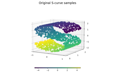
對於一個類似的範例，將這些方法應用於 S 曲線數據集，請參閱流形學習方法比較

請注意，MDS 的目的是找到數據的低維表示（此處為 2D），其中距離能很好地尊重原始高維空間中的距離，與其他流形學習演算法不同，它不尋求在低維空間中對數據進行各向同性表示。此處的流形問題與地球的平面地圖表示非常相似，就像地圖投影一樣

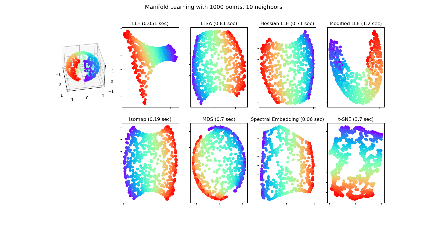
Manifold Learning with 1000 points, 10 neighbors, LLE (0.051 sec), LTSA (0.81 sec), Hessian LLE (0.71 sec), Modified LLE (1.2 sec), Isomap (0.19 sec), MDS (0.7 sec), Spectral Embedding (0.06 sec), t-SNE (3.7 sec)

standard: 0.051 sec
ltsa: 0.81 sec
hessian: 0.71 sec
modified: 1.2 sec
ISO: 0.19 sec
MDS: 0.7 sec
Spectral Embedding: 0.06 sec
t-SNE: 3.7 sec

# Authors: The scikit-learn developers
# SPDX-License-Identifier: BSD-3-Clause

from time import time

import matplotlib.pyplot as plt

# Unused but required import for doing 3d projections with matplotlib < 3.2
import mpl_toolkits.mplot3d  # noqa: F401
import numpy as np
from matplotlib.ticker import NullFormatter

from sklearn import manifold
from sklearn.utils import check_random_state

# Variables for manifold learning.
n_neighbors = 10
n_samples = 1000

# Create our sphere.
random_state = check_random_state(0)
p = random_state.rand(n_samples) * (2 * np.pi - 0.55)
t = random_state.rand(n_samples) * np.pi

# Sever the poles from the sphere.
indices = (t < (np.pi - (np.pi / 8))) & (t > ((np.pi / 8)))
colors = p[indices]
x, y, z = (
    np.sin(t[indices]) * np.cos(p[indices]),
    np.sin(t[indices]) * np.sin(p[indices]),
    np.cos(t[indices]),
)

# Plot our dataset.
fig = plt.figure(figsize=(15, 8))
plt.suptitle(
    "Manifold Learning with %i points, %i neighbors" % (1000, n_neighbors), fontsize=14
)

ax = fig.add_subplot(251, projection="3d")
ax.scatter(x, y, z, c=p[indices], cmap=plt.cm.rainbow)
ax.view_init(40, -10)

sphere_data = np.array([x, y, z]).T

# Perform Locally Linear Embedding Manifold learning
methods = ["standard", "ltsa", "hessian", "modified"]
labels = ["LLE", "LTSA", "Hessian LLE", "Modified LLE"]

for i, method in enumerate(methods):
    t0 = time()
    trans_data = (
        manifold.LocallyLinearEmbedding(
            n_neighbors=n_neighbors, n_components=2, method=method, random_state=42
        )
        .fit_transform(sphere_data)
        .T
    )
    t1 = time()
    print("%s: %.2g sec" % (methods[i], t1 - t0))

    ax = fig.add_subplot(252 + i)
    plt.scatter(trans_data[0], trans_data[1], c=colors, cmap=plt.cm.rainbow)
    plt.title("%s (%.2g sec)" % (labels[i], t1 - t0))
    ax.xaxis.set_major_formatter(NullFormatter())
    ax.yaxis.set_major_formatter(NullFormatter())
    plt.axis("tight")

# Perform Isomap Manifold learning.
t0 = time()
trans_data = (
    manifold.Isomap(n_neighbors=n_neighbors, n_components=2)
    .fit_transform(sphere_data)
    .T
)
t1 = time()
print("%s: %.2g sec" % ("ISO", t1 - t0))

ax = fig.add_subplot(257)
plt.scatter(trans_data[0], trans_data[1], c=colors, cmap=plt.cm.rainbow)
plt.title("%s (%.2g sec)" % ("Isomap", t1 - t0))
ax.xaxis.set_major_formatter(NullFormatter())
ax.yaxis.set_major_formatter(NullFormatter())
plt.axis("tight")

# Perform Multi-dimensional scaling.
t0 = time()
mds = manifold.MDS(2, max_iter=100, n_init=1, random_state=42)
trans_data = mds.fit_transform(sphere_data).T
t1 = time()
print("MDS: %.2g sec" % (t1 - t0))

ax = fig.add_subplot(258)
plt.scatter(trans_data[0], trans_data[1], c=colors, cmap=plt.cm.rainbow)
plt.title("MDS (%.2g sec)" % (t1 - t0))
ax.xaxis.set_major_formatter(NullFormatter())
ax.yaxis.set_major_formatter(NullFormatter())
plt.axis("tight")

# Perform Spectral Embedding.
t0 = time()
se = manifold.SpectralEmbedding(
    n_components=2, n_neighbors=n_neighbors, random_state=42
)
trans_data = se.fit_transform(sphere_data).T
t1 = time()
print("Spectral Embedding: %.2g sec" % (t1 - t0))

ax = fig.add_subplot(259)
plt.scatter(trans_data[0], trans_data[1], c=colors, cmap=plt.cm.rainbow)
plt.title("Spectral Embedding (%.2g sec)" % (t1 - t0))
ax.xaxis.set_major_formatter(NullFormatter())
ax.yaxis.set_major_formatter(NullFormatter())
plt.axis("tight")

# Perform t-distributed stochastic neighbor embedding.
t0 = time()
tsne = manifold.TSNE(n_components=2, random_state=0)
trans_data = tsne.fit_transform(sphere_data).T
t1 = time()
print("t-SNE: %.2g sec" % (t1 - t0))

ax = fig.add_subplot(2, 5, 10)
plt.scatter(trans_data[0], trans_data[1], c=colors, cmap=plt.cm.rainbow)
plt.title("t-SNE (%.2g sec)" % (t1 - t0))
ax.xaxis.set_major_formatter(NullFormatter())
ax.yaxis.set_major_formatter(NullFormatter())
plt.axis("tight")

plt.show()