注意
前往結尾下載完整的範例程式碼。或透過 JupyterLite 或 Binder 在您的瀏覽器中執行此範例
高斯過程迴歸:基本入門範例#
以兩種不同方式計算的簡單一維迴歸範例
無雜訊情況
每個資料點具有已知雜訊水平的雜訊情況
在這兩種情況下,核心的參數都是使用最大概似原理估計的。
這些圖說明了高斯過程模型的內插性質,以及其以逐點 95% 信賴區間形式呈現的機率性質。
請注意,alpha 是一個參數,用於控制假設訓練點共變異數矩陣上的 Tikhonov 正規化強度。
# Authors: The scikit-learn developers
# SPDX-License-Identifier: BSD-3-Clause
資料集產生#
我們將從產生合成資料集開始。真實的產生過程定義為 \(f(x) = x \sin(x)\)。
import numpy as np

X = np.linspace(start=0, stop=10, num=1_000).reshape(-1, 1)
y = np.squeeze(X * np.sin(X))
import matplotlib.pyplot as plt

plt.plot(X, y, label=r"$f(x) = x \sin(x)$", linestyle="dotted")
plt.legend()
plt.xlabel("$x$")
plt.ylabel("$f(x)$")
_ = plt.title("True generative process")
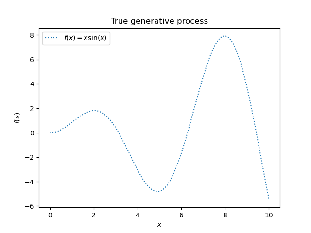
我們將在下一個實驗中使用此資料集來說明高斯過程迴歸如何運作。
無雜訊目標的範例#
在第一個範例中,我們將使用真實的產生過程,而不添加任何雜訊。對於訓練高斯過程迴歸,我們只會選擇少數樣本。
rng = np.random.RandomState(1)
training_indices = rng.choice(np.arange(y.size), size=6, replace=False)
X_train, y_train = X[training_indices], y[training_indices]
現在,我們將高斯過程擬合到這些少數訓練資料樣本上。我們將使用徑向基底函數 (RBF) 核心和常數參數來擬合振幅。
from sklearn.gaussian_process import GaussianProcessRegressor
from sklearn.gaussian_process.kernels import RBF

kernel = 1 * RBF(length_scale=1.0, length_scale_bounds=(1e-2, 1e2))
gaussian_process = GaussianProcessRegressor(kernel=kernel, n_restarts_optimizer=9)
gaussian_process.fit(X_train, y_train)
gaussian_process.kernel_
5.02**2 * RBF(length_scale=1.43)
在擬合我們的模型後,我們看到核心的超參數已最佳化。現在,我們將使用我們的核心來計算完整資料集的平均預測,並繪製 95% 信賴區間。
mean_prediction, std_prediction = gaussian_process.predict(X, return_std=True)

plt.plot(X, y, label=r"$f(x) = x \sin(x)$", linestyle="dotted")
plt.scatter(X_train, y_train, label="Observations")
plt.plot(X, mean_prediction, label="Mean prediction")
plt.fill_between(
    X.ravel(),
    mean_prediction - 1.96 * std_prediction,
    mean_prediction + 1.96 * std_prediction,
    alpha=0.5,
    label=r"95% confidence interval",
)
plt.legend()
plt.xlabel("$x$")
plt.ylabel("$f(x)$")
_ = plt.title("Gaussian process regression on noise-free dataset")
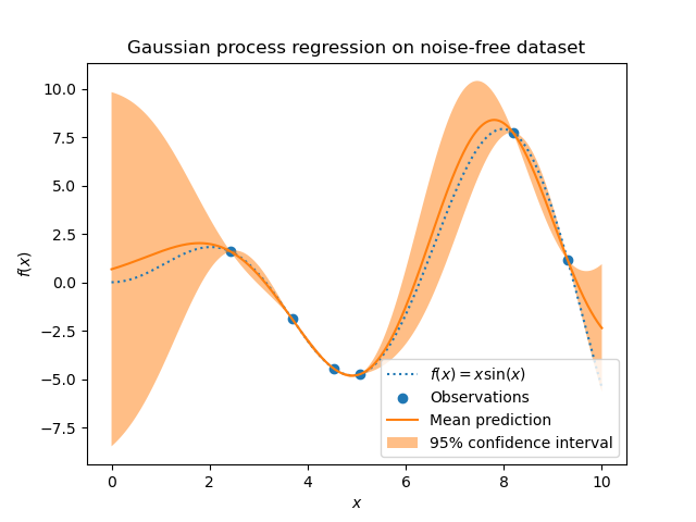
我們看到,對於在接近訓練集資料點上進行的預測,95% 信賴度的振幅很小。每當樣本遠離訓練資料時,我們模型的預測就不那麼準確,而模型預測也不那麼精確(不確定性較高)。
具有雜訊目標的範例#
我們可以重複類似的實驗,這次在目標中加入額外的雜訊。這將允許看到雜訊對擬合模型的影響。
我們在目標中添加一些具有任意標準差的隨機高斯雜訊。
noise_std = 0.75
y_train_noisy = y_train + rng.normal(loc=0.0, scale=noise_std, size=y_train.shape)
我們建立類似的高斯過程模型。除了核心之外,這次我們還指定了參數 alpha,該參數可以解釋為高斯雜訊的變異數。
gaussian_process = GaussianProcessRegressor(
    kernel=kernel, alpha=noise_std**2, n_restarts_optimizer=9
)
gaussian_process.fit(X_train, y_train_noisy)
mean_prediction, std_prediction = gaussian_process.predict(X, return_std=True)
讓我們像之前一樣繪製平均預測和不確定性區域。
plt.plot(X, y, label=r"$f(x) = x \sin(x)$", linestyle="dotted")
plt.errorbar(
    X_train,
    y_train_noisy,
    noise_std,
    linestyle="None",
    color="tab:blue",
    marker=".",
    markersize=10,
    label="Observations",
)
plt.plot(X, mean_prediction, label="Mean prediction")
plt.fill_between(
    X.ravel(),
    mean_prediction - 1.96 * std_prediction,
    mean_prediction + 1.96 * std_prediction,
    color="tab:orange",
    alpha=0.5,
    label=r"95% confidence interval",
)
plt.legend()
plt.xlabel("$x$")
plt.ylabel("$f(x)$")
_ = plt.title("Gaussian process regression on a noisy dataset")
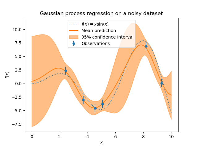
雜訊會影響接近訓練樣本的預測:由於我們明確地為給定的水平目標雜訊建模,因此與輸入變數無關,訓練樣本附近預測的不確定性較大。
腳本的總執行時間:(0 分鐘 0.509 秒)
相關範例