流形學習方法的比較#

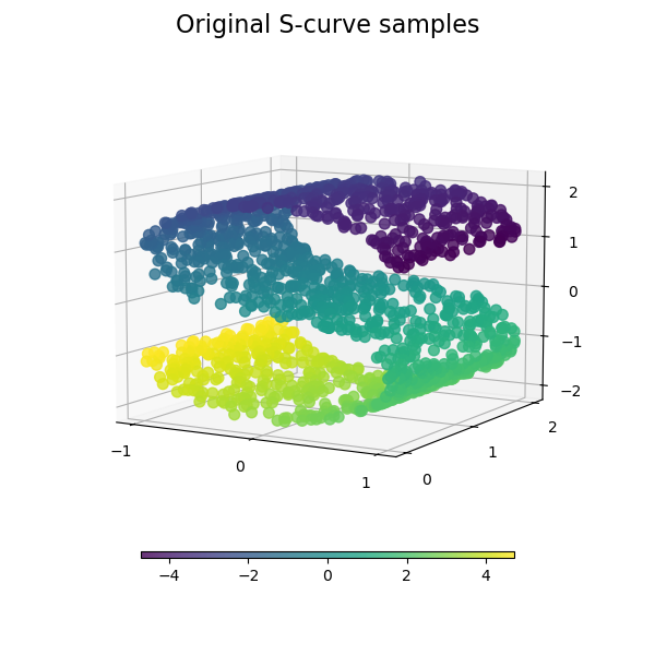
使用各種流形學習方法在 S 曲線資料集上進行降維的圖示。

有關這些演算法的討論和比較，請參閱流形模組頁面

對於一個類似的範例，其中這些方法應用於球體資料集，請參閱在分割球體上的流形學習方法

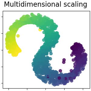
請注意，MDS 的目的是尋找資料的低維度表示 (此處為 2D)，其中距離與原始高維度空間中的距離相符，與其他流形學習演算法不同，它不會在低維度空間中尋求資料的同向性表示。

# Authors: The scikit-learn developers
# SPDX-License-Identifier: BSD-3-Clause

資料集準備#

我們先產生 S 曲線資料集。

import matplotlib.pyplot as plt

# unused but required import for doing 3d projections with matplotlib < 3.2
import mpl_toolkits.mplot3d  # noqa: F401
from matplotlib import ticker

from sklearn import datasets, manifold

n_samples = 1500
S_points, S_color = datasets.make_s_curve(n_samples, random_state=0)

讓我們看一下原始資料。同時定義一些輔助函數，我們將在後面使用它們。

def plot_3d(points, points_color, title):
    x, y, z = points.T

    fig, ax = plt.subplots(
        figsize=(6, 6),
        facecolor="white",
        tight_layout=True,
        subplot_kw={"projection": "3d"},
    )
    fig.suptitle(title, size=16)
    col = ax.scatter(x, y, z, c=points_color, s=50, alpha=0.8)
    ax.view_init(azim=-60, elev=9)
    ax.xaxis.set_major_locator(ticker.MultipleLocator(1))
    ax.yaxis.set_major_locator(ticker.MultipleLocator(1))
    ax.zaxis.set_major_locator(ticker.MultipleLocator(1))

    fig.colorbar(col, ax=ax, orientation="horizontal", shrink=0.6, aspect=60, pad=0.01)
    plt.show()


def plot_2d(points, points_color, title):
    fig, ax = plt.subplots(figsize=(3, 3), facecolor="white", constrained_layout=True)
    fig.suptitle(title, size=16)
    add_2d_scatter(ax, points, points_color)
    plt.show()


def add_2d_scatter(ax, points, points_color, title=None):
    x, y = points.T
    ax.scatter(x, y, c=points_color, s=50, alpha=0.8)
    ax.set_title(title)
    ax.xaxis.set_major_formatter(ticker.NullFormatter())
    ax.yaxis.set_major_formatter(ticker.NullFormatter())


plot_3d(S_points, S_color, "Original S-curve samples")

定義流形學習的演算法#

流形學習是一種非線性降維的方法。此任務的演算法基於這樣一個觀念，即許多資料集的維度僅是人為地高。

在使用者指南中閱讀更多內容。

n_neighbors = 12  # neighborhood which is used to recover the locally linear structure
n_components = 2  # number of coordinates for the manifold

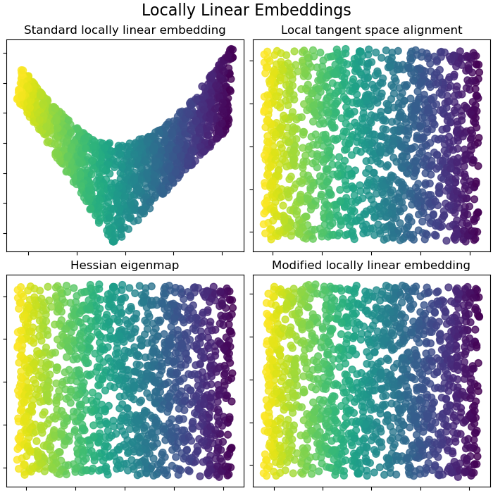
局部線性嵌入#

局部線性嵌入 (LLE) 可以被認為是一系列局部主成分分析，這些分析會在全域比較以找到最佳的非線性嵌入。在使用者指南中閱讀更多內容。

params = {
    "n_neighbors": n_neighbors,
    "n_components": n_components,
    "eigen_solver": "auto",
    "random_state": 0,
}

lle_standard = manifold.LocallyLinearEmbedding(method="standard", **params)
S_standard = lle_standard.fit_transform(S_points)

lle_ltsa = manifold.LocallyLinearEmbedding(method="ltsa", **params)
S_ltsa = lle_ltsa.fit_transform(S_points)

lle_hessian = manifold.LocallyLinearEmbedding(method="hessian", **params)
S_hessian = lle_hessian.fit_transform(S_points)

lle_mod = manifold.LocallyLinearEmbedding(method="modified", **params)
S_mod = lle_mod.fit_transform(S_points)

fig, axs = plt.subplots(
    nrows=2, ncols=2, figsize=(7, 7), facecolor="white", constrained_layout=True
)
fig.suptitle("Locally Linear Embeddings", size=16)

lle_methods = [
    ("Standard locally linear embedding", S_standard),
    ("Local tangent space alignment", S_ltsa),
    ("Hessian eigenmap", S_hessian),
    ("Modified locally linear embedding", S_mod),
]
for ax, method in zip(axs.flat, lle_methods):
    name, points = method
    add_2d_scatter(ax, points, S_color, name)

plt.show()

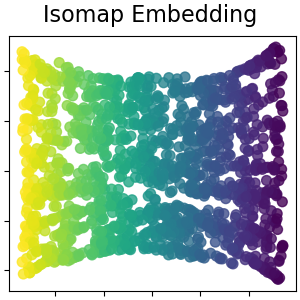
Locally Linear Embeddings, Standard locally linear embedding, Local tangent space alignment, Hessian eigenmap, Modified locally linear embedding

Isomap 嵌入#

透過等距映射進行非線性降維。Isomap 尋求一種較低維度的嵌入，以保持所有點之間的測地距離。在使用者指南中閱讀更多內容。

isomap = manifold.Isomap(n_neighbors=n_neighbors, n_components=n_components, p=1)
S_isomap = isomap.fit_transform(S_points)

plot_2d(S_isomap, S_color, "Isomap Embedding")

多維縮放#

多維縮放 (MDS) 尋求資料的低維度表示，其中距離與原始高維度空間中的距離相符。在使用者指南中閱讀更多內容。

md_scaling = manifold.MDS(
    n_components=n_components,
    max_iter=50,
    n_init=4,
    random_state=0,
    normalized_stress=False,
)
S_scaling = md_scaling.fit_transform(S_points)

plot_2d(S_scaling, S_color, "Multidimensional scaling")

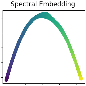
用於非線性降維的光譜嵌入#

此實作使用拉普拉斯本徵映射，該映射使用圖拉普拉斯的頻譜分解來尋找資料的低維度表示。在使用者指南中閱讀更多內容。

spectral = manifold.SpectralEmbedding(
    n_components=n_components, n_neighbors=n_neighbors, random_state=42
)
S_spectral = spectral.fit_transform(S_points)

plot_2d(S_spectral, S_color, "Spectral Embedding")

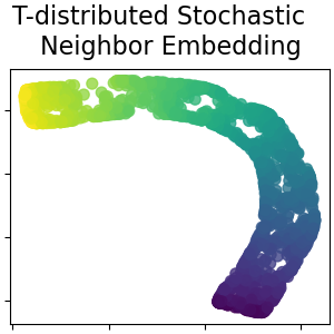
T 分佈隨機鄰近嵌入#

它將資料點之間的相似性轉換為聯合機率，並嘗試最小化低維度嵌入的聯合機率與高維度資料的聯合機率之間的 Kullback-Leibler 散度。t-SNE 有一個非凸的成本函數，也就是說，使用不同的初始化，我們可能會得到不同的結果。在使用者指南中閱讀更多內容。

t_sne = manifold.TSNE(
    n_components=n_components,
    perplexity=30,
    init="random",
    max_iter=250,
    random_state=0,
)
S_t_sne = t_sne.fit_transform(S_points)

plot_2d(S_t_sne, S_color, "T-distributed Stochastic  \n Neighbor Embedding")