注意
前往結尾以下載完整的範例程式碼。或透過 JupyterLite 或 Binder 在您的瀏覽器中執行此範例
機器學習無法推斷因果關係#
機器學習模型非常適合測量統計關聯。不幸的是,除非我們願意對資料做出強烈的假設,否則這些模型無法推斷因果關係。
為了說明這一點,我們將模擬一種情況,在這種情況下,我們嘗試回答教育經濟學中最重要的一個問題:獲得大學學位對時薪的因果影響是什麼? 儘管這個問題的答案對政策制定者至關重要,但遺漏變數偏差 (OVB) 阻礙了我們確定這種因果影響。
# Authors: The scikit-learn developers
# SPDX-License-Identifier: BSD-3-Clause
資料集:模擬的時薪#
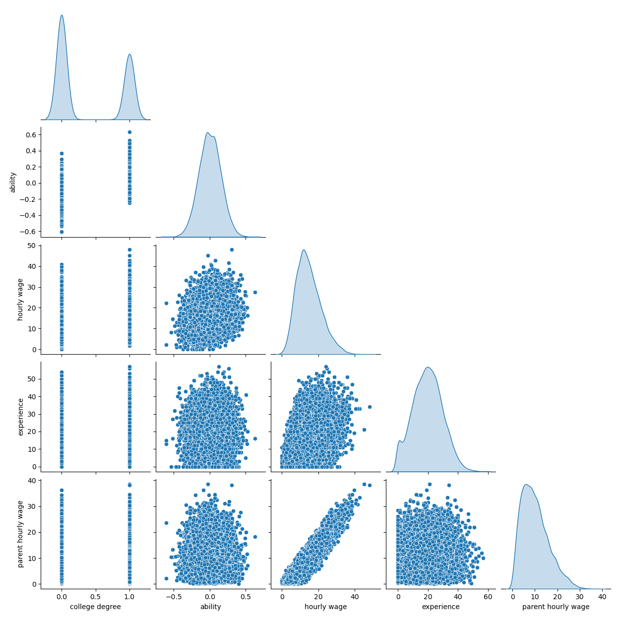
資料產生過程在下面的程式碼中列出。工作經驗 (以年為單位) 和能力衡量標準是從常態分佈中提取的;其中一位父母的時薪是從 Beta 分佈中提取的。然後,我們建立一個大學學位的指標,該指標受到能力和父母時薪的正面影響。最後,我們將時薪建模為所有先前變數的線性函數和一個隨機成分。請注意,所有變數對時薪都有正面影響。
import numpy as np
import pandas as pd

n_samples = 10_000
rng = np.random.RandomState(32)

experiences = rng.normal(20, 10, size=n_samples).astype(int)
experiences[experiences < 0] = 0
abilities = rng.normal(0, 0.15, size=n_samples)
parent_hourly_wages = 50 * rng.beta(2, 8, size=n_samples)
parent_hourly_wages[parent_hourly_wages < 0] = 0
college_degrees = (
    9 * abilities + 0.02 * parent_hourly_wages + rng.randn(n_samples) > 0.7
).astype(int)

true_coef = pd.Series(
    {
        "college degree": 2.0,
        "ability": 5.0,
        "experience": 0.2,
        "parent hourly wage": 1.0,
    }
)
hourly_wages = (
    true_coef["experience"] * experiences
    + true_coef["parent hourly wage"] * parent_hourly_wages
    + true_coef["college degree"] * college_degrees
    + true_coef["ability"] * abilities
    + rng.normal(0, 1, size=n_samples)
)

hourly_wages[hourly_wages < 0] = 0
模擬資料的描述#
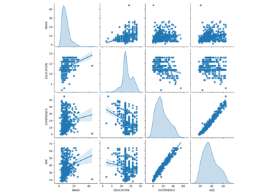
下圖顯示了每個變數的分佈,以及成對的散佈圖。我們的 OVB 故事的關鍵是能力和大學學位之間的正面關係。
import seaborn as sns

df = pd.DataFrame(
    {
        "college degree": college_degrees,
        "ability": abilities,
        "hourly wage": hourly_wages,
        "experience": experiences,
        "parent hourly wage": parent_hourly_wages,
    }
)

grid = sns.pairplot(df, diag_kind="kde", corner=True)
在下一節中,我們訓練預測模型,因此我們將目標欄與所有特徵分開,並將資料分成訓練集和測試集。
from sklearn.model_selection import train_test_split

target_name = "hourly wage"
X, y = df.drop(columns=target_name), df[target_name]
X_train, X_test, y_train, y_test = train_test_split(X, y, test_size=0.2, random_state=0)
使用完全觀察到的變數進行收入預測#
首先,我們訓練一個預測模型,一個LinearRegression模型。在這個實驗中,我們假設真實生成模型使用的所有變數都是可用的。
from sklearn.linear_model import LinearRegression
from sklearn.metrics import r2_score
features_names = ["experience", "parent hourly wage", "college degree", "ability"]
regressor_with_ability = LinearRegression()
regressor_with_ability.fit(X_train[features_names], y_train)
y_pred_with_ability = regressor_with_ability.predict(X_test[features_names])
R2_with_ability = r2_score(y_test, y_pred_with_ability)
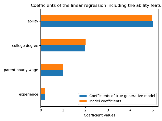
print(f"R2 score with ability: {R2_with_ability:.3f}")
R2 score with ability: 0.975
此模型可以很好地預測時薪,如高的 R2 分數所示。我們繪製模型係數,以顯示我們精確地恢復了真實生成模型的值。
import matplotlib.pyplot as plt

model_coef = pd.Series(regressor_with_ability.coef_, index=features_names)
coef = pd.concat(
    [true_coef[features_names], model_coef],
    keys=["Coefficients of true generative model", "Model coefficients"],
    axis=1,
)
ax = coef.plot.barh()
ax.set_xlabel("Coefficient values")
ax.set_title("Coefficients of the linear regression including the ability features")
_ = plt.tight_layout()
使用部分觀察結果進行收入預測#
實際上,智力能力並未被觀察到,或者僅從無意中也衡量教育程度的代理變數中估計(例如,透過智商測驗)。但是,在線性模型中省略「能力」特徵會透過正 OVB 膨脹估計值。
features_names = ["experience", "parent hourly wage", "college degree"]

regressor_without_ability = LinearRegression()
regressor_without_ability.fit(X_train[features_names], y_train)
y_pred_without_ability = regressor_without_ability.predict(X_test[features_names])
R2_without_ability = r2_score(y_test, y_pred_without_ability)

print(f"R2 score without ability: {R2_without_ability:.3f}")
R2 score without ability: 0.968
當我們在 R2 分數方面省略能力特徵時,模型的預測能力類似。我們現在檢查模型的係數是否與真實生成模型不同。
model_coef = pd.Series(regressor_without_ability.coef_, index=features_names)
coef = pd.concat(
    [true_coef[features_names], model_coef],
    keys=["Coefficients of true generative model", "Model coefficients"],
    axis=1,
)
ax = coef.plot.barh()
ax.set_xlabel("Coefficient values")
_ = ax.set_title("Coefficients of the linear regression excluding the ability feature")
plt.tight_layout()
plt.show()
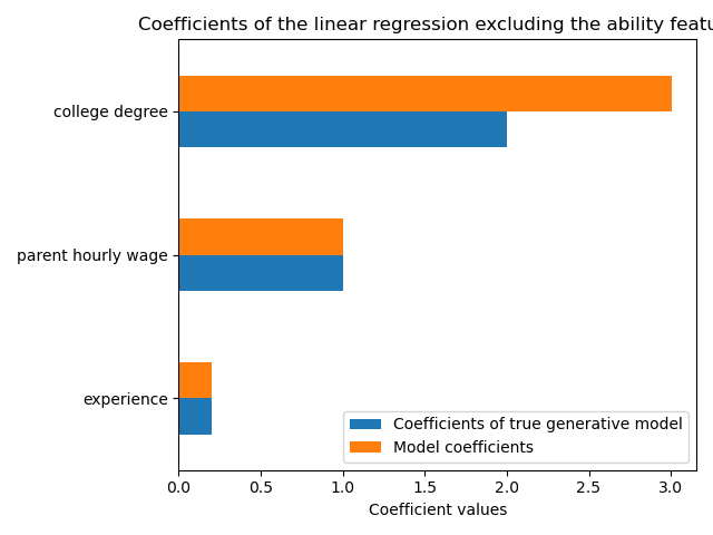
為了補償遺漏的變數,模型會膨脹大學學位特徵的係數。因此,將此係數值解釋為真實生成模型的因果影響是不正確的。
經驗教訓#
機器學習模型並非為估計因果影響而設計。雖然我們用線性模型展示了這一點,但 OVB 會影響任何類型的模型。
每當解釋係數或由於其中一個特徵的變化而引起的預測變化時,請務必記住可能未被觀察到的變數,這些變數可能與所討論的特徵和目標變數都相關。這些變數稱為混淆變數。為了在存在混淆的情況下仍然估計因果關係,研究人員通常會進行實驗,其中處理變數(例如大學學位)是隨機的。當實驗過於昂貴或不道德時,研究人員有時可以使用其他因果推論技術,例如工具變數 (IV) 估計。
指令碼總執行時間:(0 分鐘 2.721 秒)
相關範例