注意
跳至結尾以下載完整的範例程式碼。或透過 JupyterLite 或 Binder 在您的瀏覽器中執行此範例
scikit-learn 1.4 的版本重點#
我們很高興宣佈 scikit-learn 1.4 的發布!新增了許多錯誤修復和改進,以及一些新的主要功能。我們在下面詳細介紹此版本的一些主要功能。**如需所有變更的詳盡清單**,請參閱版本說明。
要安裝最新版本(使用 pip)
pip install --upgrade scikit-learn
或使用 conda
conda install -c conda-forge scikit-learn
HistGradientBoosting 原生支援 DataFrames 中的類別 DTypes#
ensemble.HistGradientBoostingClassifier 和 ensemble.HistGradientBoostingRegressor 現在直接支援具有類別特徵的資料框架。這裡我們有一個混合了類別和數值特徵的資料集
from sklearn.datasets import fetch_openml

X_adult, y_adult = fetch_openml("adult", version=2, return_X_y=True)

# Remove redundant and non-feature columns
X_adult = X_adult.drop(["education-num", "fnlwgt"], axis="columns")
X_adult.dtypes
age                  int64
workclass         category
education         category
marital-status    category
occupation        category
relationship      category
race              category
sex               category
capital-gain         int64
capital-loss         int64
hours-per-week       int64
native-country    category
dtype: object
透過設定 categorical_features="from_dtype",梯度提升分類器會將具有類別 dtypes 的列視為演算法中的類別特徵
from sklearn.ensemble import HistGradientBoostingClassifier
from sklearn.model_selection import train_test_split
from sklearn.metrics import roc_auc_score

X_train, X_test, y_train, y_test = train_test_split(X_adult, y_adult, random_state=0)
hist = HistGradientBoostingClassifier(categorical_features="from_dtype")

hist.fit(X_train, y_train)
y_decision = hist.decision_function(X_test)
print(f"ROC AUC score is {roc_auc_score(y_test, y_decision)}")
ROC AUC score is 0.9290956815049027
set_output 中的 Polars 輸出#
scikit-learn 的轉換器現在透過 set_output API 支援 polars 輸出。
import polars as pl
from sklearn.preprocessing import StandardScaler
from sklearn.preprocessing import OneHotEncoder
from sklearn.compose import ColumnTransformer

df = pl.DataFrame(
    {"height": [120, 140, 150, 110, 100], "pet": ["dog", "cat", "dog", "cat", "cat"]}
)
preprocessor = ColumnTransformer(
    [
        ("numerical", StandardScaler(), ["height"]),
        ("categorical", OneHotEncoder(sparse_output=False), ["pet"]),
    ],
    verbose_feature_names_out=False,
)
preprocessor.set_output(transform="polars")

df_out = preprocessor.fit_transform(df)
df_out
print(f"Output type: {type(df_out)}")
Output type: <class 'polars.dataframe.frame.DataFrame'>
隨機森林的遺失值支援#
類別 ensemble.RandomForestClassifier 和 ensemble.RandomForestRegressor 現在支援遺失值。在訓練每棵個別樹時,分割器會評估每個潛在的閾值,讓遺失值進入左節點和右節點。更多詳細資訊請參閱使用者指南。
import numpy as np
from sklearn.ensemble import RandomForestClassifier

X = np.array([0, 1, 6, np.nan]).reshape(-1, 1)
y = [0, 0, 1, 1]

forest = RandomForestClassifier(random_state=0).fit(X, y)
forest.predict(X)
array([0, 0, 1, 1])
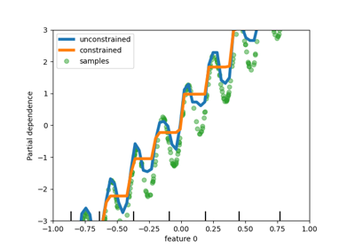
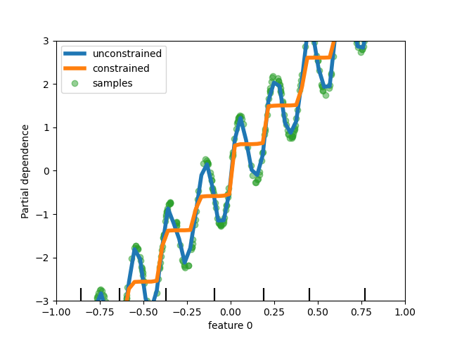
在基於樹的模型中新增對單調約束的支援#
雖然我們在 scikit-learn 0.23 中為基於直方圖的梯度提升新增了對單調約束的支援,但我們現在為所有其他基於樹的模型(如樹、隨機森林、極端樹和精確梯度提升)支援此功能。在這裡,我們展示此功能在迴歸問題上的隨機森林應用。
import matplotlib.pyplot as plt
from sklearn.inspection import PartialDependenceDisplay
from sklearn.ensemble import RandomForestRegressor

n_samples = 500
rng = np.random.RandomState(0)
X = rng.randn(n_samples, 2)
noise = rng.normal(loc=0.0, scale=0.01, size=n_samples)
y = 5 * X[:, 0] + np.sin(10 * np.pi * X[:, 0]) - noise

rf_no_cst = RandomForestRegressor().fit(X, y)
rf_cst = RandomForestRegressor(monotonic_cst=[1, 0]).fit(X, y)

disp = PartialDependenceDisplay.from_estimator(
    rf_no_cst,
    X,
    features=[0],
    feature_names=["feature 0"],
    line_kw={"linewidth": 4, "label": "unconstrained", "color": "tab:blue"},
)
PartialDependenceDisplay.from_estimator(
    rf_cst,
    X,
    features=[0],
    line_kw={"linewidth": 4, "label": "constrained", "color": "tab:orange"},
    ax=disp.axes_,
)
disp.axes_[0, 0].plot(
    X[:, 0], y, "o", alpha=0.5, zorder=-1, label="samples", color="tab:green"
)
disp.axes_[0, 0].set_ylim(-3, 3)
disp.axes_[0, 0].set_xlim(-1, 1)
disp.axes_[0, 0].legend()
plt.show()
豐富的估計器顯示#
估計器顯示已豐富化:如果我們看一下上面定義的 forest
forest
可以透過點擊圖表右上角的「?」圖示來存取估計器的文件。
此外,當估計器擬合時,顯示會從橘色變為藍色。您也可以將滑鼠游標停在「i」圖示上來取得此資訊。
from sklearn.base import clone

clone(forest)  # the clone is not fitted
中繼資料路由支援#
許多中繼估計器和交叉驗證常式現在支援中繼資料路由,這些都列在使用者指南中。例如,這是您如何使用樣本權重和 GroupKFold 進行巢狀交叉驗證的方式
import sklearn
from sklearn.metrics import get_scorer
from sklearn.datasets import make_regression
from sklearn.linear_model import Lasso
from sklearn.model_selection import GridSearchCV, cross_validate, GroupKFold

# For now by default metadata routing is disabled, and need to be explicitly
# enabled.
sklearn.set_config(enable_metadata_routing=True)

n_samples = 100
X, y = make_regression(n_samples=n_samples, n_features=5, noise=0.5)
rng = np.random.RandomState(7)
groups = rng.randint(0, 10, size=n_samples)
sample_weights = rng.rand(n_samples)
estimator = Lasso().set_fit_request(sample_weight=True)
hyperparameter_grid = {"alpha": [0.1, 0.5, 1.0, 2.0]}
scoring_inner_cv = get_scorer("neg_mean_squared_error").set_score_request(
    sample_weight=True
)
inner_cv = GroupKFold(n_splits=5)

grid_search = GridSearchCV(
    estimator=estimator,
    param_grid=hyperparameter_grid,
    cv=inner_cv,
    scoring=scoring_inner_cv,
)

outer_cv = GroupKFold(n_splits=5)
scorers = {
    "mse": get_scorer("neg_mean_squared_error").set_score_request(sample_weight=True)
}
results = cross_validate(
    grid_search,
    X,
    y,
    cv=outer_cv,
    scoring=scorers,
    return_estimator=True,
    params={"sample_weight": sample_weights, "groups": groups},
)
print("cv error on test sets:", results["test_mse"])

# Setting the flag to the default `False` to avoid interference with other
# scripts.
sklearn.set_config(enable_metadata_routing=False)
cv error on test sets: [-0.33164913 -0.35912565 -0.30811173 -0.15610822 -0.25797037]
改善稀疏資料上 PCA 的記憶體和執行時間效率#
PCA 現在能夠透過利用 scipy.sparse.linalg.LinearOperator 原生處理 arpack 求解器的稀疏矩陣,以避免在執行資料集共變數矩陣的特徵值分解時具體化大型稀疏矩陣。
from sklearn.decomposition import PCA
import scipy.sparse as sp
from time import time

X_sparse = sp.random(m=1000, n=1000, random_state=0)
X_dense = X_sparse.toarray()

t0 = time()
PCA(n_components=10, svd_solver="arpack").fit(X_sparse)
time_sparse = time() - t0

t0 = time()
PCA(n_components=10, svd_solver="arpack").fit(X_dense)
time_dense = time() - t0

print(f"Speedup: {time_dense / time_sparse:.1f}x")
Speedup: 3.7x
腳本的總執行時間:(0 分鐘 2.082 秒)
相關範例