注意事項
前往結尾以下載完整的範例程式碼。或透過 JupyterLite 或 Binder 在您的瀏覽器中執行此範例
直方圖梯度提升樹中的特徵#
基於直方圖的梯度提升 (HGBT) 模型可能是 scikit-learn 中最有用的監督學習模型之一。它們基於一種現代的梯度提升實作,可與 LightGBM 和 XGBoost 相媲美。因此,HGBT 模型比隨機森林等替代模型具有更豐富的功能,且效能通常更高,尤其是在樣本數量大於數萬個時(請參閱比較隨機森林和直方圖梯度提升模型)。
HGBT 模型最重要的可用性特徵為
此範例旨在展示所有要點,除了第 2 和第 6 點在真實生活場景中的應用。
# Authors: The scikit-learn developers
# SPDX-License-Identifier: BSD-3-Clause
準備資料#
電力資料集包含從澳洲新南威爾斯電力市場收集的資料。在此市場中,價格並非固定,而是受供需影響。它們每五分鐘設定一次。往返鄰近的維多利亞州的電力傳輸旨在減輕波動。
此資料集最初名為 ELEC2,包含 1996 年 5 月 7 日至 1998 年 12 月 5 日的 45,312 個執行個體。資料集的每個樣本都參照 30 分鐘的時間段,即每天的每個時間段都有 48 個執行個體。資料集上的每個樣本都有 7 個資料行
日期:介於 1996 年 5 月 7 日至 1998 年 12 月 5 日之間。介於 0 到 1 之間正規化;
星期幾:星期幾(1-7);
期間:超過 24 小時的半小時間隔。介於 0 到 1 之間正規化;
nswprice/nswdemand:新南威爾斯的電力價格/需求;
vicprice/vicdemand:維多利亞州的電力價格/需求。
最初,它是一項分類任務,但在此我們使用它來進行迴歸任務,以預測各州之間排定的電力傳輸。
from sklearn.datasets import fetch_openml

electricity = fetch_openml(
    name="electricity", version=1, as_frame=True, parser="pandas"
)
df = electricity.frame
此特定資料集在前 17,760 個樣本中具有逐步常數目標
df["transfer"][:17_760].unique()
array([0.414912, 0.500526])
讓我們刪除這些項目,並探索一週中不同日期的每小時電力傳輸
import matplotlib.pyplot as plt
import seaborn as sns

df = electricity.frame.iloc[17_760:]
X = df.drop(columns=["transfer", "class"])
y = df["transfer"]

fig, ax = plt.subplots(figsize=(15, 10))
pointplot = sns.lineplot(x=df["period"], y=df["transfer"], hue=df["day"], ax=ax)
handles, lables = ax.get_legend_handles_labels()
ax.set(
    title="Hourly energy transfer for different days of the week",
    xlabel="Normalized time of the day",
    ylabel="Normalized energy transfer",
)
_ = ax.legend(handles, ["Sun", "Mon", "Tue", "Wed", "Thu", "Fri", "Sat"])
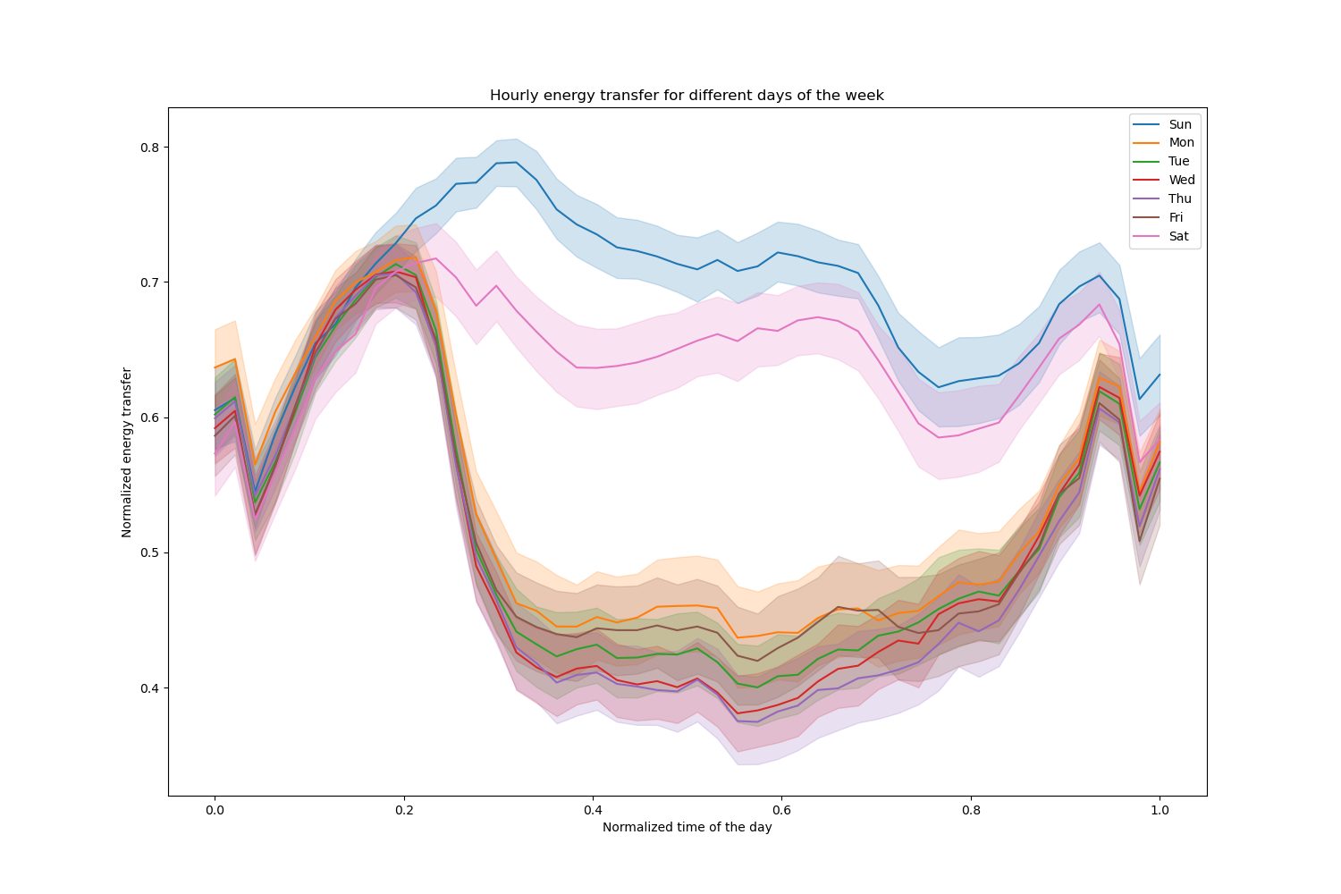
請注意,週末的能量傳輸會系統性地增加。
樹狀結構數量和提早停止的影響#
為了說明(最大)樹狀結構數量的影響,我們使用整個資料集訓練每日電力傳輸的HistGradientBoostingRegressor。然後,我們根據 max_iter 參數視覺化其預測。在此,我們不嘗試評估模型的效能及其泛化能力,而是評估其從訓練資料中學習的能力。
from sklearn.ensemble import HistGradientBoostingRegressor
from sklearn.model_selection import train_test_split

X_train, X_test, y_train, y_test = train_test_split(X, y, test_size=0.4, shuffle=False)

print(f"Training sample size: {X_train.shape[0]}")
print(f"Test sample size: {X_test.shape[0]}")
print(f"Number of features: {X_train.shape[1]}")
Training sample size: 16531
Test sample size: 11021
Number of features: 7
max_iter_list = [5, 50]
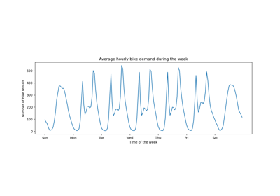
average_week_demand = (
df.loc[X_test.index].groupby(["day", "period"], observed=False)["transfer"].mean()
)
colors = sns.color_palette("colorblind")
fig, ax = plt.subplots(figsize=(10, 5))
average_week_demand.plot(color=colors[0], label="recorded average", linewidth=2, ax=ax)
for idx, max_iter in enumerate(max_iter_list):
hgbt = HistGradientBoostingRegressor(
max_iter=max_iter, categorical_features=None, random_state=42
)
hgbt.fit(X_train, y_train)
y_pred = hgbt.predict(X_test)
prediction_df = df.loc[X_test.index].copy()
prediction_df["y_pred"] = y_pred
average_pred = prediction_df.groupby(["day", "period"], observed=False)[
"y_pred"
].mean()
average_pred.plot(
color=colors[idx + 1], label=f"max_iter={max_iter}", linewidth=2, ax=ax
)
ax.set(
title="Predicted average energy transfer during the week",
xticks=[(i + 0.2) * 48 for i in range(7)],
xticklabels=["Sun", "Mon", "Tue", "Wed", "Thu", "Fri", "Sat"],
xlabel="Time of the week",
ylabel="Normalized energy transfer",
)
_ = ax.legend()
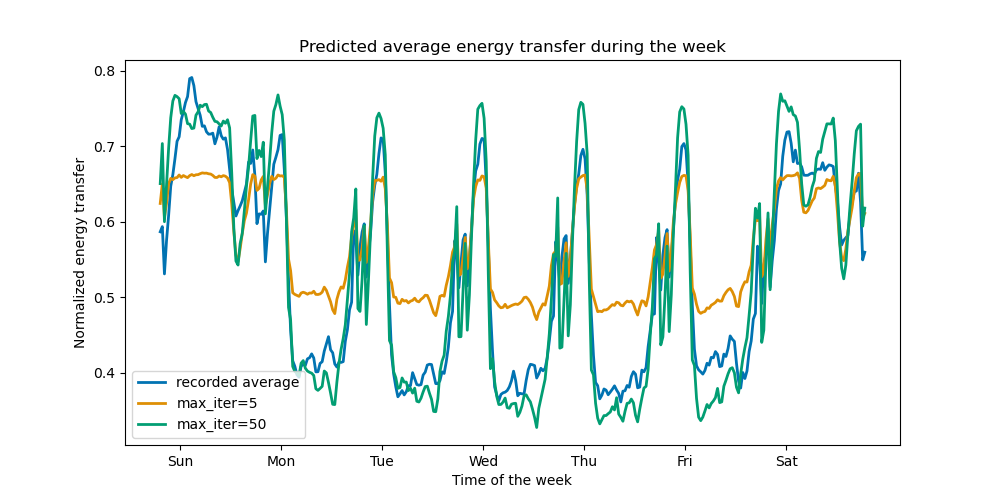
僅需幾次迭代,HGBT 模型即可實現收斂(請參閱比較隨機森林和直方圖梯度提升模型),這表示新增更多樹狀結構不會再改善模型。在上圖中,5 次迭代不足以獲得良好的預測。經過 50 次迭代,我們已經能夠做得很好。
將 max_iter 設定得太高可能會降低預測品質,並耗費大量可避免的運算資源。因此,scikit-learn 中的 HGBT 實作提供自動提早停止策略。透過此策略,模型會使用一小部分的訓練資料作為內部驗證集 (validation_fraction),如果驗證分數在 n_iter_no_change 次迭代後未改善(或降低),則會停止訓練,直到達到特定容差 (tol)。
請注意,learning_rate 和 max_iter 之間存在權衡:一般而言,較小的學習速率較佳,但需要更多迭代才能收斂到最小損失,而較大的學習速率會更快收斂(需要較少的迭代/樹狀結構),但會犧牲較大的最小損失。
由於學習速率和迭代次數之間存在高度相關性,因此良好的做法是調整學習速率以及所有(重要的)其他超參數,將 HBGT 擬合到訓練集,並為 max_iter 使用足夠大的值,並透過提早停止和某些明確的 validation_fraction 來判斷最佳 max_iter。
common_params = {
    "max_iter": 1_000,
    "learning_rate": 0.3,
    "validation_fraction": 0.2,
    "random_state": 42,
    "categorical_features": None,
    "scoring": "neg_root_mean_squared_error",
}

hgbt = HistGradientBoostingRegressor(early_stopping=True, **common_params)
hgbt.fit(X_train, y_train)

_, ax = plt.subplots()
plt.plot(-hgbt.validation_score_)
_ = ax.set(
    xlabel="number of iterations",
    ylabel="root mean squared error",
    title=f"Loss of hgbt with early stopping (n_iter={hgbt.n_iter_})",
)
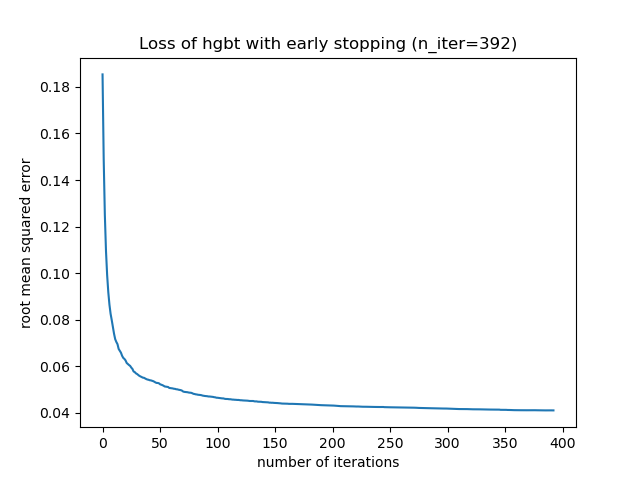
然後,我們可以將 max_iter 的值覆寫為合理的值,並避免內部驗證的額外運算成本。向上捨入迭代次數可能會考慮訓練集的變異性
import math

common_params["max_iter"] = math.ceil(hgbt.n_iter_ / 100) * 100
common_params["early_stopping"] = False
hgbt = HistGradientBoostingRegressor(**common_params)
注意事項
在提早停止期間完成的內部驗證對於時間序列來說並非最佳。
支援遺失值#
HGBT 模型原生支援遺失值。在訓練期間,樹狀結構成長器會根據潛在的增益,決定在每次分割時,具有遺失值的樣本應該往左子節點還是右子節點移動。在預測時,這些樣本會相應地被送到學習到的子節點。如果一個特徵在訓練期間沒有遺失值,那麼在預測時,該特徵具有遺失值的樣本會被送到具有最多樣本的子節點(如在擬合期間所見)。
本範例展示 HGBT 回歸如何處理完全隨機遺失 (MCAR) 的值,即遺失與觀察到的資料或未觀察到的資料無關。我們可以透過隨機將隨機選取特徵的值替換為 nan 值來模擬這種情況。
import numpy as np

from sklearn.metrics import root_mean_squared_error

rng = np.random.RandomState(42)
first_week = slice(0, 336)  # first week in the test set as 7 * 48 = 336
missing_fraction_list = [0, 0.01, 0.03]


def generate_missing_values(X, missing_fraction):
    total_cells = X.shape[0] * X.shape[1]
    num_missing_cells = int(total_cells * missing_fraction)
    row_indices = rng.choice(X.shape[0], num_missing_cells, replace=True)
    col_indices = rng.choice(X.shape[1], num_missing_cells, replace=True)
    X_missing = X.copy()
    X_missing.iloc[row_indices, col_indices] = np.nan
    return X_missing


fig, ax = plt.subplots(figsize=(12, 6))
ax.plot(y_test.values[first_week], label="Actual transfer")

for missing_fraction in missing_fraction_list:
    X_train_missing = generate_missing_values(X_train, missing_fraction)
    X_test_missing = generate_missing_values(X_test, missing_fraction)
    hgbt.fit(X_train_missing, y_train)
    y_pred = hgbt.predict(X_test_missing[first_week])
    rmse = root_mean_squared_error(y_test[first_week], y_pred)
    ax.plot(
        y_pred[first_week],
        label=f"missing_fraction={missing_fraction}, RMSE={rmse:.3f}",
        alpha=0.5,
    )
ax.set(
    title="Daily energy transfer predictions on data with MCAR values",
    xticks=[(i + 0.2) * 48 for i in range(7)],
    xticklabels=["Mon", "Tue", "Wed", "Thu", "Fri", "Sat", "Sun"],
    xlabel="Time of the week",
    ylabel="Normalized energy transfer",
)
_ = ax.legend(loc="lower right")
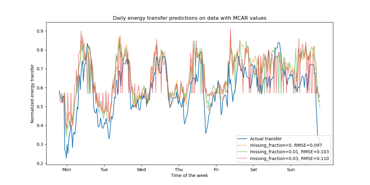
如預期,隨著遺失值比例的增加,模型效能會下降。
支援分位數損失#
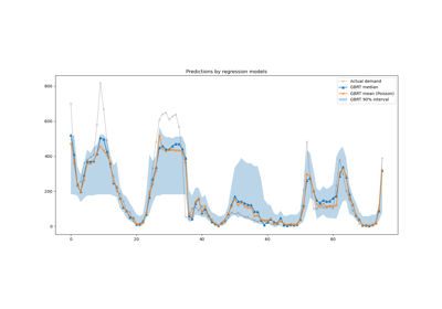
回歸中的分位數損失可以觀察目標變數的變異性或不確定性。例如,預測第 5 個和第 95 個百分位數可以提供 90% 的預測區間,即我們預期新的觀察值以 90% 的機率落入的範圍。
from sklearn.metrics import mean_pinball_loss

quantiles = [0.95, 0.05]
predictions = []

fig, ax = plt.subplots(figsize=(12, 6))
ax.plot(y_test.values[first_week], label="Actual transfer")

for quantile in quantiles:
    hgbt_quantile = HistGradientBoostingRegressor(
        loss="quantile", quantile=quantile, **common_params
    )
    hgbt_quantile.fit(X_train, y_train)
    y_pred = hgbt_quantile.predict(X_test[first_week])

    predictions.append(y_pred)
    score = mean_pinball_loss(y_test[first_week], y_pred)
    ax.plot(
        y_pred[first_week],
        label=f"quantile={quantile}, pinball loss={score:.2f}",
        alpha=0.5,
    )

ax.fill_between(
    range(len(predictions[0][first_week])),
    predictions[0][first_week],
    predictions[1][first_week],
    color=colors[0],
    alpha=0.1,
)
ax.set(
    title="Daily energy transfer predictions with quantile loss",
    xticks=[(i + 0.2) * 48 for i in range(7)],
    xticklabels=["Mon", "Tue", "Wed", "Thu", "Fri", "Sat", "Sun"],
    xlabel="Time of the week",
    ylabel="Normalized energy transfer",
)
_ = ax.legend(loc="lower right")
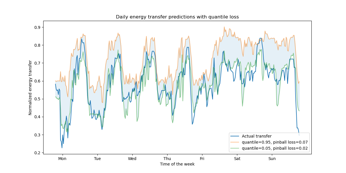
我們觀察到高估能量轉移的趨勢。這可以透過計算經驗覆蓋率數值來定量確認,如信賴區間校準章節中所做的那樣。請記住,那些預測的百分位數僅是來自模型的估計值。仍然可以透過以下方式提高此類估計的品質:
收集更多數據點;
更好地調整模型超參數,請參閱梯度提升回歸的預測區間;
從相同的數據設計更多具預測性的特徵,請參閱時間相關的特徵工程。
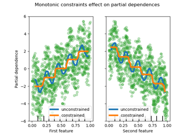
單調約束#
如果特定的領域知識要求特徵和目標之間的關係是單調遞增或遞減的,則可以使用單調約束在 HGBT 模型的預測中強制執行這種行為。這使得模型更易於解釋,並可以降低其變異數(並可能緩解過擬合),但可能會增加偏差。單調約束也可以用於強制執行特定的監管要求、確保合規性並符合道德考量。
在本範例中,從維多利亞州向新南威爾斯州轉移能源的政策旨在緩解價格波動,這意味著模型預測必須強制執行此目標,即轉移應隨著新南威爾斯州的價格和需求增加,但也要隨著維多利亞州的價格和需求減少,以使兩地居民受益。
如果訓練資料具有特徵名稱,則可以使用以下約定傳遞字典來指定單調約束
1:單調遞增
0:無約束
-1:單調遞減
或者,可以傳遞一個類似陣列的物件,按位置編碼上述約定。
from sklearn.inspection import PartialDependenceDisplay

monotonic_cst = {
    "date": 0,
    "day": 0,
    "period": 0,
    "nswdemand": 1,
    "nswprice": 1,
    "vicdemand": -1,
    "vicprice": -1,
}
hgbt_no_cst = HistGradientBoostingRegressor(
    categorical_features=None, random_state=42
).fit(X, y)
hgbt_cst = HistGradientBoostingRegressor(
    monotonic_cst=monotonic_cst, categorical_features=None, random_state=42
).fit(X, y)

fig, ax = plt.subplots(nrows=2, figsize=(15, 10))
disp = PartialDependenceDisplay.from_estimator(
    hgbt_no_cst,
    X,
    features=["nswdemand", "nswprice"],
    line_kw={"linewidth": 2, "label": "unconstrained", "color": "tab:blue"},
    ax=ax[0],
)
PartialDependenceDisplay.from_estimator(
    hgbt_cst,
    X,
    features=["nswdemand", "nswprice"],
    line_kw={"linewidth": 2, "label": "constrained", "color": "tab:orange"},
    ax=disp.axes_,
)
disp = PartialDependenceDisplay.from_estimator(
    hgbt_no_cst,
    X,
    features=["vicdemand", "vicprice"],
    line_kw={"linewidth": 2, "label": "unconstrained", "color": "tab:blue"},
    ax=ax[1],
)
PartialDependenceDisplay.from_estimator(
    hgbt_cst,
    X,
    features=["vicdemand", "vicprice"],
    line_kw={"linewidth": 2, "label": "constrained", "color": "tab:orange"},
    ax=disp.axes_,
)
_ = plt.legend()
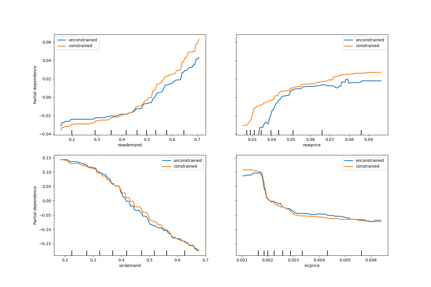
請注意,nswdemand 和 vicdemand 看起來在沒有約束的情況下已經是單調的。這是一個很好的例子,說明具有單調性約束的模型是「過度約束」的。
此外,我們可以驗證引入單調約束並未顯著降低模型的預測品質。為此,我們使用 TimeSeriesSplit 交叉驗證來估計測試分數的變異數。這樣做可以保證訓練資料不會晚於測試資料,這在處理具有時間關係的資料時至關重要。
from sklearn.metrics import make_scorer, root_mean_squared_error
from sklearn.model_selection import TimeSeriesSplit, cross_validate

ts_cv = TimeSeriesSplit(n_splits=5, gap=48, test_size=336)  # a week has 336 samples
scorer = make_scorer(root_mean_squared_error)

cv_results = cross_validate(hgbt_no_cst, X, y, cv=ts_cv, scoring=scorer)
rmse = cv_results["test_score"]
print(f"RMSE without constraints = {rmse.mean():.3f} +/- {rmse.std():.3f}")

cv_results = cross_validate(hgbt_cst, X, y, cv=ts_cv, scoring=scorer)
rmse = cv_results["test_score"]
print(f"RMSE with constraints    = {rmse.mean():.3f} +/- {rmse.std():.3f}")
RMSE without constraints = 0.103 +/- 0.030
RMSE with constraints    = 0.107 +/- 0.034
話雖如此,請注意,比較的是兩個不同的模型,它們可能透過不同的超參數組合進行最佳化。這就是為什麼我們沒有像之前那樣在此章節中使用 common_params 的原因。
腳本的總執行時間:(0 分 22.516 秒)
相關範例