比較玩具資料集上離群值偵測的異常偵測演算法#

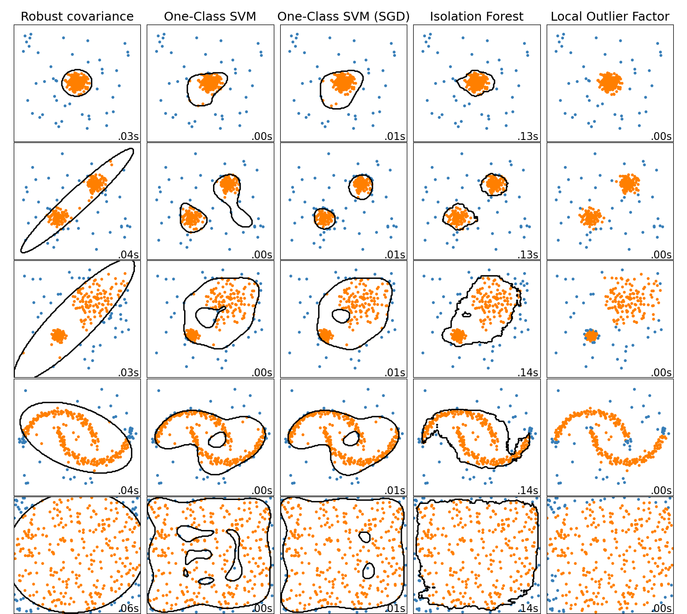
此範例顯示不同異常偵測演算法在 2D 資料集上的特性。資料集包含一個或兩個模式（高密度區域），以說明演算法處理多模態資料的能力。

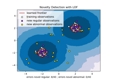
對於每個資料集，15% 的樣本會產生為隨機均勻雜訊。此比例是給定給 OneClassSVM 的 nu 參數和其他離群值偵測演算法的汙染參數的值。除了局部離群因子 (LOF) 外，內點和離群值之間的決策邊界以黑色顯示，因為當 LOF 用於離群值偵測時，它沒有可以應用於新資料的預測方法。

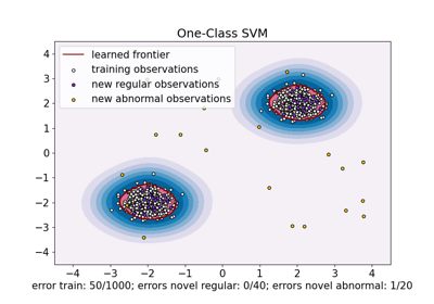
已知 OneClassSVM 對離群值敏感，因此在離群值偵測方面表現不佳。此估計器最適合在訓練集未受離群值汙染時進行新奇偵測。也就是說，在高維度或在沒有對內點資料分佈的任何假設的情況下進行離群值偵測非常具有挑戰性，並且在這些情況下，單類別 SVM 可能會根據其超參數的值產生有用的結果。

sklearn.linear_model.SGDOneClassSVM 是基於隨機梯度下降 (SGD) 的單類別 SVM 的實作。結合核心近似，此估計器可用於逼近核心化 sklearn.svm.OneClassSVM 的解。我們注意到，雖然不完全相同，但 sklearn.linear_model.SGDOneClassSVM 和 sklearn.svm.OneClassSVM 的決策邊界非常相似。使用 sklearn.linear_model.SGDOneClassSVM 的主要優點是它會隨樣本數量線性縮放。

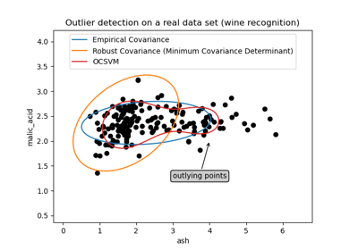
sklearn.covariance.EllipticEnvelope 假設資料是高斯的並學習一個橢圓。因此，當資料不是單模態時，它會降級。但是請注意，此估計器對離群值具有穩健性。

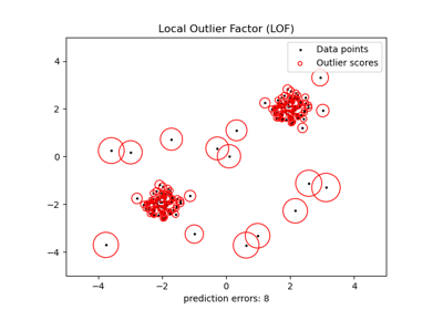
IsolationForest 和 LocalOutlierFactor 似乎在多模態資料集上表現相當不錯。LocalOutlierFactor 相較於其他估計器的優點顯示在第三個資料集中，其中兩個模式具有不同的密度。此優點由 LOF 的局部特性來解釋，這表示它僅將一個樣本的異常分數與其鄰居的分數進行比較。

最後，對於最後一個資料集，很難說一個樣本比另一個樣本更異常，因為它們均勻分佈在超立方體中。除了稍微過擬合的 OneClassSVM 之外，所有估計器都為這種情況提供了不錯的解決方案。在這種情況下，明智之舉是更仔細地查看樣本的異常分數，因為好的估計器應該將相似的分數指派給所有樣本。

雖然這些範例提供了一些關於演算法的直覺，但這種直覺可能不適用於非常高維度的資料。

最後，請注意，此處模型的參數是手動挑選的，但在實踐中需要調整。在沒有標籤資料的情況下，問題是完全無監督的，因此模型選擇可能是一個挑戰。

Robust covariance, One-Class SVM, One-Class SVM (SGD), Isolation Forest, Local Outlier Factor

# Authors: The scikit-learn developers
# SPDX-License-Identifier: BSD-3-Clause

import time

import matplotlib
import matplotlib.pyplot as plt
import numpy as np

from sklearn import svm
from sklearn.covariance import EllipticEnvelope
from sklearn.datasets import make_blobs, make_moons
from sklearn.ensemble import IsolationForest
from sklearn.kernel_approximation import Nystroem
from sklearn.linear_model import SGDOneClassSVM
from sklearn.neighbors import LocalOutlierFactor
from sklearn.pipeline import make_pipeline

matplotlib.rcParams["contour.negative_linestyle"] = "solid"

# Example settings
n_samples = 300
outliers_fraction = 0.15
n_outliers = int(outliers_fraction * n_samples)
n_inliers = n_samples - n_outliers

# define outlier/anomaly detection methods to be compared.
# the SGDOneClassSVM must be used in a pipeline with a kernel approximation
# to give similar results to the OneClassSVM
anomaly_algorithms = [
    (
        "Robust covariance",
        EllipticEnvelope(contamination=outliers_fraction, random_state=42),
    ),
    ("One-Class SVM", svm.OneClassSVM(nu=outliers_fraction, kernel="rbf", gamma=0.1)),
    (
        "One-Class SVM (SGD)",
        make_pipeline(
            Nystroem(gamma=0.1, random_state=42, n_components=150),
            SGDOneClassSVM(
                nu=outliers_fraction,
                shuffle=True,
                fit_intercept=True,
                random_state=42,
                tol=1e-6,
            ),
        ),
    ),
    (
        "Isolation Forest",
        IsolationForest(contamination=outliers_fraction, random_state=42),
    ),
    (
        "Local Outlier Factor",
        LocalOutlierFactor(n_neighbors=35, contamination=outliers_fraction),
    ),
]

# Define datasets
blobs_params = dict(random_state=0, n_samples=n_inliers, n_features=2)
datasets = [
    make_blobs(centers=[[0, 0], [0, 0]], cluster_std=0.5, **blobs_params)[0],
    make_blobs(centers=[[2, 2], [-2, -2]], cluster_std=[0.5, 0.5], **blobs_params)[0],
    make_blobs(centers=[[2, 2], [-2, -2]], cluster_std=[1.5, 0.3], **blobs_params)[0],
    4.0
    * (
        make_moons(n_samples=n_samples, noise=0.05, random_state=0)[0]
        - np.array([0.5, 0.25])
    ),
    14.0 * (np.random.RandomState(42).rand(n_samples, 2) - 0.5),
]

# Compare given classifiers under given settings
xx, yy = np.meshgrid(np.linspace(-7, 7, 150), np.linspace(-7, 7, 150))

plt.figure(figsize=(len(anomaly_algorithms) * 2 + 4, 12.5))
plt.subplots_adjust(
    left=0.02, right=0.98, bottom=0.001, top=0.96, wspace=0.05, hspace=0.01
)

plot_num = 1
rng = np.random.RandomState(42)

for i_dataset, X in enumerate(datasets):
    # Add outliers
    X = np.concatenate([X, rng.uniform(low=-6, high=6, size=(n_outliers, 2))], axis=0)

    for name, algorithm in anomaly_algorithms:
        t0 = time.time()
        algorithm.fit(X)
        t1 = time.time()
        plt.subplot(len(datasets), len(anomaly_algorithms), plot_num)
        if i_dataset == 0:
            plt.title(name, size=18)

        # fit the data and tag outliers
        if name == "Local Outlier Factor":
            y_pred = algorithm.fit_predict(X)
        else:
            y_pred = algorithm.fit(X).predict(X)

        # plot the levels lines and the points
        if name != "Local Outlier Factor":  # LOF does not implement predict
            Z = algorithm.predict(np.c_[xx.ravel(), yy.ravel()])
            Z = Z.reshape(xx.shape)
            plt.contour(xx, yy, Z, levels=[0], linewidths=2, colors="black")

        colors = np.array(["#377eb8", "#ff7f00"])
        plt.scatter(X[:, 0], X[:, 1], s=10, color=colors[(y_pred + 1) // 2])

        plt.xlim(-7, 7)
        plt.ylim(-7, 7)
        plt.xticks(())
        plt.yticks(())
        plt.text(
            0.99,
            0.01,
            ("%.2fs" % (t1 - t0)).lstrip("0"),
            transform=plt.gca().transAxes,
            size=15,
            horizontalalignment="right",
        )
        plot_num += 1

plt.show()