scikit-learn 1.3 的版本重點#

我們很高興宣布 scikit-learn 1.3 的發布！新增了許多錯誤修復和改進，以及一些新的關鍵功能。我們在下面詳細介紹此版本的一些主要功能。如需所有變更的完整列表，請參閱版本說明。

安裝最新版本（使用 pip）

pip install --upgrade scikit-learn

或使用 conda

conda install -c conda-forge scikit-learn

中繼資料路由#

我們正在引入一種新的方式來路由中繼資料，例如程式碼庫中的 sample_weight，這會影響諸如 pipeline.Pipeline 和 model_selection.GridSearchCV 等元估算器如何路由中繼資料。雖然此功能的基础結構已包含在此版本中，但工作仍在進行中，並非所有元估算器都支援此新功能。您可以在中繼資料路由使用者指南中閱讀有關此功能的更多資訊。請注意，此功能仍在開發中，且尚未在大多數元估算器中實作。

第三方開發人員可以開始將其納入其元估算器中。如需更多詳細資訊，請參閱中繼資料路由開發人員指南。

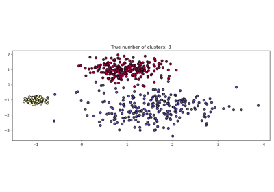
HDBSCAN：階層式基於密度的叢集#

最初託管在 scikit-learn-contrib 儲存庫中，cluster.HDBSCAN 已被採用到 scikit-learn 中。它缺少原始實作中的一些功能，這些功能將在未來的版本中新增。透過同時對多個 epsilon 值執行 cluster.DBSCAN 的修改版本，cluster.HDBSCAN 可找到不同密度的叢集，使其比 cluster.DBSCAN 更能抵抗參數選擇。更多詳細資訊請參閱使用者指南。

import numpy as np
from sklearn.cluster import HDBSCAN
from sklearn.datasets import load_digits
from sklearn.metrics import v_measure_score

X, true_labels = load_digits(return_X_y=True)
print(f"number of digits: {len(np.unique(true_labels))}")

hdbscan = HDBSCAN(min_cluster_size=15).fit(X)
non_noisy_labels = hdbscan.labels_[hdbscan.labels_ != -1]
print(f"number of clusters found: {len(np.unique(non_noisy_labels))}")

print(v_measure_score(true_labels[hdbscan.labels_ != -1], non_noisy_labels))

number of digits: 10
number of clusters found: 11
0.9694898472080092

TargetEncoder：一種新的類別編碼策略#

非常適合具有高基數的類別特徵，preprocessing.TargetEncoder 根據屬於該類別的觀測值的平均目標值的縮減估計值來編碼類別。更多詳細資訊請參閱使用者指南。

import numpy as np
from sklearn.preprocessing import TargetEncoder

X = np.array([["cat"] * 30 + ["dog"] * 20 + ["snake"] * 38], dtype=object).T
y = [90.3] * 30 + [20.4] * 20 + [21.2] * 38

enc = TargetEncoder(random_state=0)
X_trans = enc.fit_transform(X, y)

enc.encodings_

[array([90.3, 20.4, 21.2])]

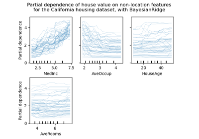
決策樹中支援遺失值#

類別 tree.DecisionTreeClassifier 和 tree.DecisionTreeRegressor 現在支援遺失值。對於非遺失資料上的每個潛在閾值，分割器將評估所有遺失值轉到左節點或右節點的分割。請參閱使用者指南中的更多詳細資訊，或參閱直方圖梯度提升樹中的特徵，以取得 HistGradientBoostingRegressor 中此功能的用例範例。

import numpy as np
from sklearn.tree import DecisionTreeClassifier

X = np.array([0, 1, 6, np.nan]).reshape(-1, 1)
y = [0, 0, 1, 1]

tree = DecisionTreeClassifier(random_state=0).fit(X, y)
tree.predict(X)

array([0, 0, 1, 1])

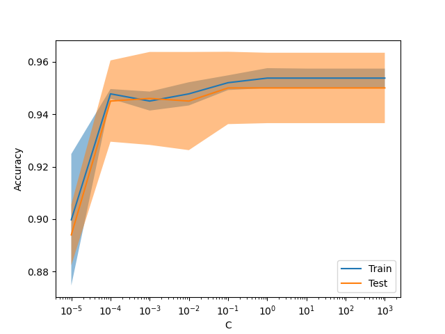
新的顯示 `ValidationCurveDisplay`#

現在可以使用 model_selection.ValidationCurveDisplay 繪製 model_selection.validation_curve 的結果。

from sklearn.datasets import make_classification
from sklearn.linear_model import LogisticRegression
from sklearn.model_selection import ValidationCurveDisplay

X, y = make_classification(1000, 10, random_state=0)

_ = ValidationCurveDisplay.from_estimator(
    LogisticRegression(),
    X,
    y,
    param_name="C",
    param_range=np.geomspace(1e-5, 1e3, num=9),
    score_type="both",
    score_name="Accuracy",
)

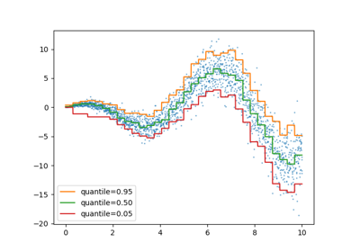
梯度提升的伽瑪損失#

類別 ensemble.HistGradientBoostingRegressor 透過 loss="gamma" 支援 Gamma 偏差損失函數。此損失函數適用於對具有右偏分佈的嚴格正目標進行建模。

import numpy as np
from sklearn.model_selection import cross_val_score
from sklearn.datasets import make_low_rank_matrix
from sklearn.ensemble import HistGradientBoostingRegressor

n_samples, n_features = 500, 10
rng = np.random.RandomState(0)
X = make_low_rank_matrix(n_samples, n_features, random_state=rng)
coef = rng.uniform(low=-10, high=20, size=n_features)
y = rng.gamma(shape=2, scale=np.exp(X @ coef) / 2)
gbdt = HistGradientBoostingRegressor(loss="gamma")
cross_val_score(gbdt, X, y).mean()

np.float64(0.46858513287221654)

在 `OrdinalEncoder` 中分組不頻繁的類別#

與 preprocessing.OneHotEncoder 類似，類別 preprocessing.OrdinalEncoder 現在支援將不頻繁的類別聚合成每個特徵的單一輸出。啟用不頻繁類別聚合的參數是 min_frequency 和 max_categories。請參閱使用者指南以獲取更多詳細資訊。

from sklearn.preprocessing import OrdinalEncoder
import numpy as np

X = np.array(
    [["dog"] * 5 + ["cat"] * 20 + ["rabbit"] * 10 + ["snake"] * 3], dtype=object
).T
enc = OrdinalEncoder(min_frequency=6).fit(X)
enc.infrequent_categories_