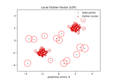
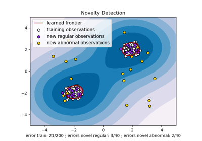
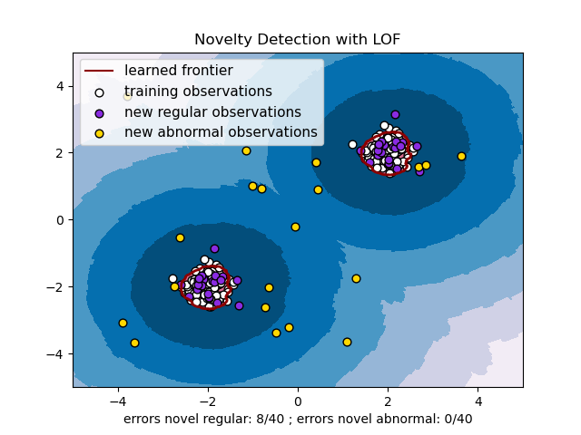
使用局部離群因子 (LOF) 進行新奇檢測#

局部離群因子 (LOF) 演算法是一種非監督異常檢測方法，它計算相對於其鄰居的給定資料點的局部密度偏差。它將密度顯著低於其鄰居的樣本視為離群值。此範例說明如何使用 LOF 進行新奇檢測。請注意，當 LOF 用於新奇檢測時，您**絕對不能**在訓練集上使用 predict、decision_function 和 score_samples，因為這會導致錯誤的結果。您必須僅在新的未見資料 (不在訓練集中) 上使用這些方法。有關離群值檢測和新奇檢測之間的差異以及如何使用 LOF 進行離群值檢測的詳細資訊，請參閱使用者指南。

考慮的鄰居數量（參數 n_neighbors）通常設定為：1) 大於叢集必須包含的最小樣本數，以便其他樣本相對於此叢集成為局部離群值，以及 2) 小於可能成為局部離群值的附近樣本的最大數量。實際上，通常無法獲得此類資訊，並且通常採用 n_neighbors=20 看起來效果很好。

# Authors: The scikit-learn developers
# SPDX-License-Identifier: BSD-3-Clause

import matplotlib
import matplotlib.lines as mlines
import matplotlib.pyplot as plt
import numpy as np

from sklearn.neighbors import LocalOutlierFactor

np.random.seed(42)

xx, yy = np.meshgrid(np.linspace(-5, 5, 500), np.linspace(-5, 5, 500))
# Generate normal (not abnormal) training observations
X = 0.3 * np.random.randn(100, 2)
X_train = np.r_[X + 2, X - 2]
# Generate new normal (not abnormal) observations
X = 0.3 * np.random.randn(20, 2)
X_test = np.r_[X + 2, X - 2]
# Generate some abnormal novel observations
X_outliers = np.random.uniform(low=-4, high=4, size=(20, 2))

# fit the model for novelty detection (novelty=True)
clf = LocalOutlierFactor(n_neighbors=20, novelty=True, contamination=0.1)
clf.fit(X_train)
# DO NOT use predict, decision_function and score_samples on X_train as this
# would give wrong results but only on new unseen data (not used in X_train),
# e.g. X_test, X_outliers or the meshgrid
y_pred_test = clf.predict(X_test)
y_pred_outliers = clf.predict(X_outliers)
n_error_test = y_pred_test[y_pred_test == -1].size
n_error_outliers = y_pred_outliers[y_pred_outliers == 1].size

# plot the learned frontier, the points, and the nearest vectors to the plane
Z = clf.decision_function(np.c_[xx.ravel(), yy.ravel()])
Z = Z.reshape(xx.shape)

plt.title("Novelty Detection with LOF")
plt.contourf(xx, yy, Z, levels=np.linspace(Z.min(), 0, 7), cmap=plt.cm.PuBu)
a = plt.contour(xx, yy, Z, levels=[0], linewidths=2, colors="darkred")
plt.contourf(xx, yy, Z, levels=[0, Z.max()], colors="palevioletred")

s = 40
b1 = plt.scatter(X_train[:, 0], X_train[:, 1], c="white", s=s, edgecolors="k")
b2 = plt.scatter(X_test[:, 0], X_test[:, 1], c="blueviolet", s=s, edgecolors="k")
c = plt.scatter(X_outliers[:, 0], X_outliers[:, 1], c="gold", s=s, edgecolors="k")
plt.axis("tight")
plt.xlim((-5, 5))
plt.ylim((-5, 5))
plt.legend(
    [mlines.Line2D([], [], color="darkred"), b1, b2, c],
    [
        "learned frontier",
        "training observations",
        "new regular observations",
        "new abnormal observations",
    ],
    loc="upper left",
    prop=matplotlib.font_manager.FontProperties(size=11),
)
plt.xlabel(
    "errors novel regular: %d/40 ; errors novel abnormal: %d/40"
    % (n_error_test, n_error_outliers)
)
plt.show()