多標籤分類 (Multilabel classification)

此範例模擬多標籤文件分類問題。數據集是根據以下過程隨機產生 (This example simulates a multi-label document classification problem. The dataset is generated randomly based on the following process)

• 選擇標籤數量：n ~ 泊松(n_labels) (pick the number of labels: n ~ Poisson(n_labels))

• n 次，選擇一個類別 c：c ~ 多項式(theta) (n times, choose a class c: c ~ Multinomial(theta))

• 選擇文件長度：k ~ 泊松(length) (pick the document length: k ~ Poisson(length))

• k 次，選擇一個單字：w ~ 多項式(theta_c) (k times, choose a word: w ~ Multinomial(theta_c))

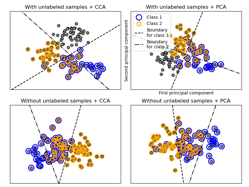
在上述過程中，使用拒絕採樣來確保 n 大於 2，且文件長度永遠不為零。同樣地，我們拒絕已經選擇的類別。分配給兩個類別的文件會以兩個有色圓圈包圍繪製 (In the above process, rejection sampling is used to make sure that n is more than 2, and that the document length is never zero. Likewise, we reject classes which have already been chosen. The documents that are assigned to both classes are plotted surrounded by two colored circles.)

分類是通過投影到 PCA 和 CCA 找到的前兩個主要成分（用於視覺化目的），然後使用 OneVsRestClassifier 元分類器，並使用兩個具有線性核函數的 SVC 來學習每個類別的判別模型來執行的。請注意，PCA 用於執行無監督降維，而 CCA 用於執行監督降維 (The classification is performed by projecting to the first two principal components found by PCA and CCA for visualisation purposes, followed by using the OneVsRestClassifier metaclassifier using two SVCs with linear kernels to learn a discriminative model for each class. Note that PCA is used to perform an unsupervised dimensionality reduction, while CCA is used to perform a supervised one.)

注意：在圖中，「未標記的樣本」並不表示我們不知道標籤（如半監督學習），而是表示樣本沒有標籤 (Note: in the plot, “unlabeled samples” does not mean that we don’t know the labels (as in semi-supervised learning) but that the samples simply do not have a label.)

# Authors: The scikit-learn developers
# SPDX-License-Identifier: BSD-3-Clause

import matplotlib.pyplot as plt
import numpy as np

from sklearn.cross_decomposition import CCA
from sklearn.datasets import make_multilabel_classification
from sklearn.decomposition import PCA
from sklearn.multiclass import OneVsRestClassifier
from sklearn.svm import SVC


def plot_hyperplane(clf, min_x, max_x, linestyle, label):
    # get the separating hyperplane
    w = clf.coef_[0]
    a = -w[0] / w[1]
    xx = np.linspace(min_x - 5, max_x + 5)  # make sure the line is long enough
    yy = a * xx - (clf.intercept_[0]) / w[1]
    plt.plot(xx, yy, linestyle, label=label)


def plot_subfigure(X, Y, subplot, title, transform):
    if transform == "pca":
        X = PCA(n_components=2).fit_transform(X)
    elif transform == "cca":
        X = CCA(n_components=2).fit(X, Y).transform(X)
    else:
        raise ValueError

    min_x = np.min(X[:, 0])
    max_x = np.max(X[:, 0])

    min_y = np.min(X[:, 1])
    max_y = np.max(X[:, 1])

    classif = OneVsRestClassifier(SVC(kernel="linear"))
    classif.fit(X, Y)

    plt.subplot(2, 2, subplot)
    plt.title(title)

    zero_class = np.where(Y[:, 0])
    one_class = np.where(Y[:, 1])
    plt.scatter(X[:, 0], X[:, 1], s=40, c="gray", edgecolors=(0, 0, 0))
    plt.scatter(
        X[zero_class, 0],
        X[zero_class, 1],
        s=160,
        edgecolors="b",
        facecolors="none",
        linewidths=2,
        label="Class 1",
    )
    plt.scatter(
        X[one_class, 0],
        X[one_class, 1],
        s=80,
        edgecolors="orange",
        facecolors="none",
        linewidths=2,
        label="Class 2",
    )

    plot_hyperplane(
        classif.estimators_[0], min_x, max_x, "k--", "Boundary\nfor class 1"
    )
    plot_hyperplane(
        classif.estimators_[1], min_x, max_x, "k-.", "Boundary\nfor class 2"
    )
    plt.xticks(())
    plt.yticks(())

    plt.xlim(min_x - 0.5 * max_x, max_x + 0.5 * max_x)
    plt.ylim(min_y - 0.5 * max_y, max_y + 0.5 * max_y)
    if subplot == 2:
        plt.xlabel("First principal component")
        plt.ylabel("Second principal component")
        plt.legend(loc="upper left")


plt.figure(figsize=(8, 6))

X, Y = make_multilabel_classification(
    n_classes=2, n_labels=1, allow_unlabeled=True, random_state=1
)

plot_subfigure(X, Y, 1, "With unlabeled samples + CCA", "cca")
plot_subfigure(X, Y, 2, "With unlabeled samples + PCA", "pca")

X, Y = make_multilabel_classification(
    n_classes=2, n_labels=1, allow_unlabeled=False, random_state=1
)

plot_subfigure(X, Y, 3, "Without unlabeled samples + CCA", "cca")
plot_subfigure(X, Y, 4, "Without unlabeled samples + PCA", "pca")

plt.subplots_adjust(0.04, 0.02, 0.97, 0.94, 0.09, 0.2)
plt.show()

相關範例 (Related examples)

比較交叉分解方法

比較交叉分解方法

繪製隨機產生的多標籤資料集

繪製隨機產生的多標籤資料集

SVM 邊界範例 (SVM Margins Example)

SVM 邊界範例 (SVM Margins Example)

半監督分類器與 Iris 數據集上的 SVM 的決策邊界 (Decision boundary of semi-supervised classifiers versus SVM on the Iris dataset)

半監督分類器與 Iris 數據集上的 SVM 的決策邊界 (Decision boundary of semi-supervised classifiers versus SVM on the Iris dataset)