注意事項
前往結尾以下載完整的範例程式碼。或透過 JupyterLite 或 Binder 在您的瀏覽器中執行此範例
事後調整決策函數的截止點#
一旦訓練完畢二元分類器,predict 方法會輸出類別標籤預測,對應於 decision_function 或 predict_proba 輸出的閾值。預設閾值定義為 0.5 的事後機率估計值或 0.0 的決策分數。然而,此預設策略對於手邊的工作可能不是最佳的。
此範例示範如何使用 TunedThresholdClassifierCV,根據感興趣的度量來調整決策閾值。
# Authors: The scikit-learn developers
# SPDX-License-Identifier: BSD-3-Clause
糖尿病資料集#
為了說明決策閾值的調整,我們將使用糖尿病資料集。此資料集可在 OpenML 上取得:https://www.openml.org/d/37。我們使用 fetch_openml 函式來提取此資料集。
from sklearn.datasets import fetch_openml

diabetes = fetch_openml(data_id=37, as_frame=True, parser="pandas")
data, target = diabetes.data, diabetes.target
我們查看目標以了解我們正在處理的問題類型。
target.value_counts()
class
tested_negative    500
tested_positive    268
Name: count, dtype: int64
我們可以發現我們正在處理二元分類問題。由於標籤未編碼為 0 和 1,我們明確表示將標記為「tested_negative」的類別視為負類別(也是最常見的類別),並將標記為「tested_positive」的類別視為正類別
neg_label, pos_label = target.value_counts().index
我們還可以觀察到,此二元問題略微不平衡,其中負類別的樣本數大約是正類別的兩倍。在評估時,我們應考慮此方面來解釋結果。
我們的原始分類器#
我們定義一個基本預測模型,由一個縮放器和一個邏輯回歸分類器組成。
from sklearn.linear_model import LogisticRegression
from sklearn.pipeline import make_pipeline
from sklearn.preprocessing import StandardScaler

model = make_pipeline(StandardScaler(), LogisticRegression())
model
我們使用交叉驗證評估我們的模型。我們使用準確度和平衡準確度來報告模型的效能。平衡準確度是一種對類別不平衡較不敏感的度量,可讓我們從長遠角度來看準確度分數。
交叉驗證可讓我們研究資料不同分割的決策閾值變異。然而,資料集相當小,使用超過 5 個摺疊來評估分散性會產生不利影響。因此,我們使用 RepeatedStratifiedKFold,其中我們應用 5 折交叉驗證的數次重複。
import pandas as pd

from sklearn.model_selection import RepeatedStratifiedKFold, cross_validate

scoring = ["accuracy", "balanced_accuracy"]
cv_scores = [
    "train_accuracy",
    "test_accuracy",
    "train_balanced_accuracy",
    "test_balanced_accuracy",
]
cv = RepeatedStratifiedKFold(n_splits=5, n_repeats=10, random_state=42)
cv_results_vanilla_model = pd.DataFrame(
    cross_validate(
        model,
        data,
        target,
        scoring=scoring,
        cv=cv,
        return_train_score=True,
        return_estimator=True,
    )
)
cv_results_vanilla_model[cv_scores].aggregate(["mean", "std"]).T
我們的預測模型成功掌握資料與目標之間的關係。訓練分數和測試分數彼此接近,這表示我們的預測模型沒有過度擬合。我們還可以觀察到,由於先前提到類別不平衡,平衡準確度低於準確度。
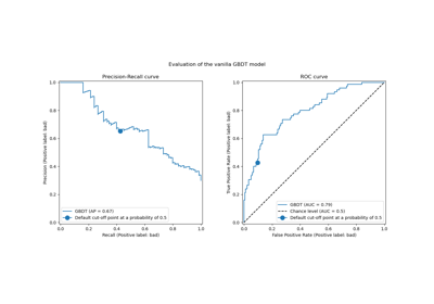
對於此分類器,我們讓決策閾值(用於將正類別的機率轉換為類別預測)設為其預設值:0.5。然而,此閾值可能不是最佳的。如果我們的目的是最大化平衡準確度,我們應選擇另一個會最大化此度量的閾值。
TunedThresholdClassifierCV 元估計器允許根據感興趣的度量調整分類器的決策閾值。
調整決策閾值#
我們建立 TunedThresholdClassifierCV 並將其設定為最大化平衡準確度。我們使用與先前相同的交叉驗證策略來評估模型。
from sklearn.model_selection import TunedThresholdClassifierCV

tuned_model = TunedThresholdClassifierCV(estimator=model, scoring="balanced_accuracy")
cv_results_tuned_model = pd.DataFrame(
    cross_validate(
        tuned_model,
        data,
        target,
        scoring=scoring,
        cv=cv,
        return_train_score=True,
        return_estimator=True,
    )
)
cv_results_tuned_model[cv_scores].aggregate(["mean", "std"]).T
與原始模型相比,我們觀察到平衡準確度分數有所提高。當然,這是以較低的準確度分數為代價的。這表示我們的模型現在對正類別更敏感,但在負類別上會犯更多錯誤。
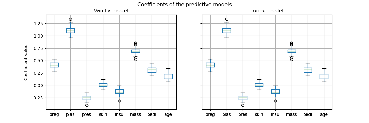
然而,請務必注意,此調整後的預測模型在內部與原始模型是相同的模型:它們具有相同的擬合係數。
import matplotlib.pyplot as plt

vanilla_model_coef = pd.DataFrame(
    [est[-1].coef_.ravel() for est in cv_results_vanilla_model["estimator"]],
    columns=diabetes.feature_names,
)
tuned_model_coef = pd.DataFrame(
    [est.estimator_[-1].coef_.ravel() for est in cv_results_tuned_model["estimator"]],
    columns=diabetes.feature_names,
)

fig, ax = plt.subplots(ncols=2, figsize=(12, 4), sharex=True, sharey=True)
vanilla_model_coef.boxplot(ax=ax[0])
ax[0].set_ylabel("Coefficient value")
ax[0].set_title("Vanilla model")
tuned_model_coef.boxplot(ax=ax[1])
ax[1].set_title("Tuned model")
_ = fig.suptitle("Coefficients of the predictive models")
在交叉驗證期間,只變更了每個模型的決策閾值。
decision_threshold = pd.Series(
    [est.best_threshold_ for est in cv_results_tuned_model["estimator"]],
)
ax = decision_threshold.plot.kde()
ax.axvline(
    decision_threshold.mean(),
    color="k",
    linestyle="--",
    label=f"Mean decision threshold: {decision_threshold.mean():.2f}",
)
ax.set_xlabel("Decision threshold")
ax.legend(loc="upper right")
_ = ax.set_title(
    "Distribution of the decision threshold \nacross different cross-validation folds"
)
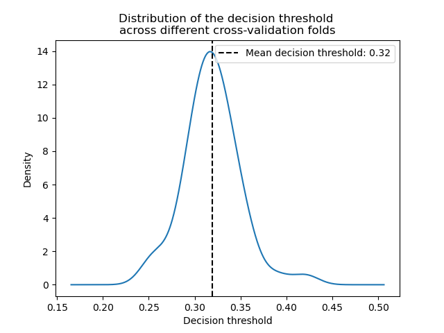
平均而言,約 0.32 的決策閾值可以最大化平衡準確率,這與預設的決策閾值 0.5 不同。因此,當使用預測模型的輸出進行決策時,調整決策閾值尤其重要。此外,用於調整決策閾值的指標應謹慎選擇。在這裡,我們使用了平衡準確率,但它可能不是當前問題最合適的指標。「正確」指標的選擇通常取決於問題本身,並且可能需要一些領域知識。請參閱標題為「針對成本敏感學習的決策閾值後調整」的範例,以了解更多詳細資訊。
腳本總運行時間: (0 分鐘 34.516 秒)
相關範例