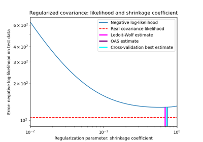
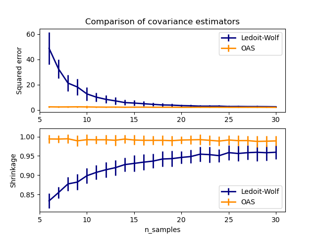
Ledoit-Wolf 與 OAS 估計#

常用的共變異數最大似然估計可以使用收縮進行正規化。Ledoit 和 Wolf 提出了一個閉合公式來計算漸近最佳收縮參數（最小化 MSE 準則），產生 Ledoit-Wolf 共變異數估計。

Chen 等人提出對 Ledoit-Wolf 收縮參數的改進，即 OAS 係數，在資料呈高斯分佈的假設下，其收斂性顯著較好。

此範例靈感來自 Chen 的出版物 [1]，顯示了使用高斯分佈資料的 LW 和 OAS 方法的估計 MSE 的比較。

[1] “Shrinkage Algorithms for MMSE Covariance Estimation” Chen et al., IEEE Trans. on Sign. Proc., Volume 58, Issue 10, October 2010.

# Authors: The scikit-learn developers
# SPDX-License-Identifier: BSD-3-Clause

import matplotlib.pyplot as plt
import numpy as np
from scipy.linalg import cholesky, toeplitz

from sklearn.covariance import OAS, LedoitWolf

np.random.seed(0)

n_features = 100
# simulation covariance matrix (AR(1) process)
r = 0.1
real_cov = toeplitz(r ** np.arange(n_features))
coloring_matrix = cholesky(real_cov)

n_samples_range = np.arange(6, 31, 1)
repeat = 100
lw_mse = np.zeros((n_samples_range.size, repeat))
oa_mse = np.zeros((n_samples_range.size, repeat))
lw_shrinkage = np.zeros((n_samples_range.size, repeat))
oa_shrinkage = np.zeros((n_samples_range.size, repeat))
for i, n_samples in enumerate(n_samples_range):
    for j in range(repeat):
        X = np.dot(np.random.normal(size=(n_samples, n_features)), coloring_matrix.T)

        lw = LedoitWolf(store_precision=False, assume_centered=True)
        lw.fit(X)
        lw_mse[i, j] = lw.error_norm(real_cov, scaling=False)
        lw_shrinkage[i, j] = lw.shrinkage_

        oa = OAS(store_precision=False, assume_centered=True)
        oa.fit(X)
        oa_mse[i, j] = oa.error_norm(real_cov, scaling=False)
        oa_shrinkage[i, j] = oa.shrinkage_

# plot MSE
plt.subplot(2, 1, 1)
plt.errorbar(
    n_samples_range,
    lw_mse.mean(1),
    yerr=lw_mse.std(1),
    label="Ledoit-Wolf",
    color="navy",
    lw=2,
)
plt.errorbar(
    n_samples_range,
    oa_mse.mean(1),
    yerr=oa_mse.std(1),
    label="OAS",
    color="darkorange",
    lw=2,
)
plt.ylabel("Squared error")
plt.legend(loc="upper right")
plt.title("Comparison of covariance estimators")
plt.xlim(5, 31)

# plot shrinkage coefficient
plt.subplot(2, 1, 2)
plt.errorbar(
    n_samples_range,
    lw_shrinkage.mean(1),
    yerr=lw_shrinkage.std(1),
    label="Ledoit-Wolf",
    color="navy",
    lw=2,
)
plt.errorbar(
    n_samples_range,
    oa_shrinkage.mean(1),
    yerr=oa_shrinkage.std(1),
    label="OAS",
    color="darkorange",
    lw=2,
)
plt.xlabel("n_samples")
plt.ylabel("Shrinkage")
plt.legend(loc="lower right")
plt.ylim(plt.ylim()[0], 1.0 + (plt.ylim()[1] - plt.ylim()[0]) / 10.0)
plt.xlim(5, 31)

plt.show()