注意
前往結尾以下載完整的範例程式碼。或透過 JupyterLite 或 Binder 在您的瀏覽器中執行此範例
時間相關特徵工程#
此筆記本介紹不同的策略,以利用時間相關特徵進行自行車共享需求迴歸任務,該任務高度依賴於商業週期(日、週、月)和年度季節週期。
在此過程中,我們介紹如何使用 sklearn.preprocessing.SplineTransformer 類別及其 extrapolation="periodic" 選項執行週期性特徵工程。
# Authors: The scikit-learn developers
# SPDX-License-Identifier: BSD-3-Clause
自行車共享需求資料集的資料探索#
我們首先從 OpenML 儲存庫載入資料。
from sklearn.datasets import fetch_openml

bike_sharing = fetch_openml("Bike_Sharing_Demand", version=2, as_frame=True)
df = bike_sharing.frame
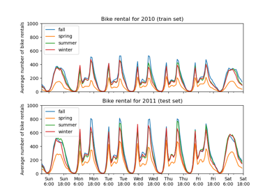
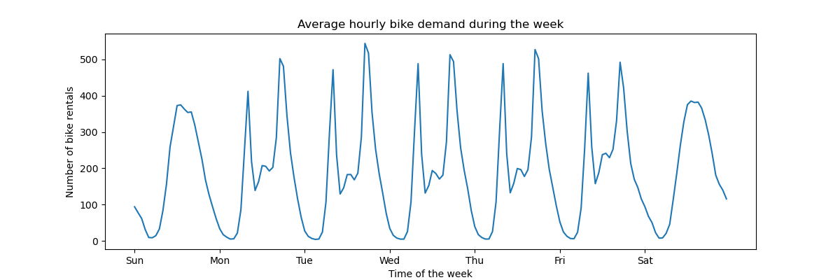
為了快速了解資料的週期性模式,讓我們看一下一週內每小時的平均需求。
請注意,一週從星期日開始,也就是週末。我們可以清楚地分辨工作日早上和晚上的通勤模式,以及週末自行車的休閒使用,其需求高峰分佈在中午左右
import matplotlib.pyplot as plt

fig, ax = plt.subplots(figsize=(12, 4))
average_week_demand = df.groupby(["weekday", "hour"])["count"].mean()
average_week_demand.plot(ax=ax)
_ = ax.set(
    title="Average hourly bike demand during the week",
    xticks=[i * 24 for i in range(7)],
    xticklabels=["Sun", "Mon", "Tue", "Wed", "Thu", "Fri", "Sat"],
    xlabel="Time of the week",
    ylabel="Number of bike rentals",
)
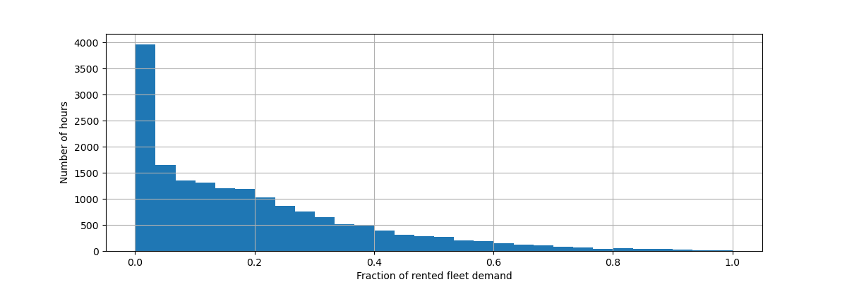
預測問題的目標是每小時自行車租賃的絕對計數
df["count"].max()
np.int64(977)
讓我們重新縮放目標變數(每小時自行車租賃數量)以預測相對需求,以便更容易將平均絕對誤差解釋為最大需求的分數。
注意
本筆記本中使用的模型之擬合方法都最小化均方誤差以估計條件均值。然而,絕對誤差會估計條件中位數。
然而,在討論中報告測試集上的效能衡量標準時,我們選擇專注於平均絕對誤差而不是(根)均方誤差,因為它更容易直觀地解釋。然而,請注意,在本研究中,一個指標的最佳模型在另一個指標方面也是最佳的。
y = df["count"] / df["count"].max()
fig, ax = plt.subplots(figsize=(12, 4))
y.hist(bins=30, ax=ax)
_ = ax.set(
    xlabel="Fraction of rented fleet demand",
    ylabel="Number of hours",
)
輸入特徵資料框架是時間註解的每小時變數記錄,描述天氣狀況。它包含數值和類別變數。請注意,時間資訊已擴展為幾個互補的欄。
X = df.drop("count", axis="columns")
X
注意
如果時間資訊僅以日期或日期時間欄的形式存在,我們可以使用 pandas 將其擴展為一天中的小時、一週中的天、一個月中的天、一年中的月份:https://pandas.dev.org.tw/pandas-docs/stable/user_guide/timeseries.html#time-date-components
我們現在檢查類別變數的分布,從 "weather" 開始
X["weather"].value_counts()
weather
clear         11413
misty          4544
rain           1419
heavy_rain        3
Name: count, dtype: int64
由於只有 3 個 "heavy_rain" 事件,我們無法使用此類別來訓練具有交叉驗證的機器學習模型。相反,我們將這些類別簡化為 "rain" 類別。
X["weather"] = (
    X["weather"]
    .astype(object)
    .replace(to_replace="heavy_rain", value="rain")
    .astype("category")
)
X["weather"].value_counts()
weather
clear    11413
misty     4544
rain      1422
Name: count, dtype: int64
正如預期的那樣,"season" 變數是平衡的
X["season"].value_counts()
season
fall      4496
summer    4409
spring    4242
winter    4232
Name: count, dtype: int64
基於時間的交叉驗證#
由於資料集是一個時間排序的事件記錄(每小時需求),我們將使用時間敏感的交叉驗證分割器來盡可能實際地評估我們的需求預測模型。我們在分割的訓練和測試端之間使用 2 天的間隔。我們還限制訓練集的大小,以使 CV 折的效能更加穩定。
1000 個測試資料點應該足以量化模型的效能。這表示略少於一個半月的連續測試資料
from sklearn.model_selection import TimeSeriesSplit

ts_cv = TimeSeriesSplit(
    n_splits=5,
    gap=48,
    max_train_size=10000,
    test_size=1000,
)
讓我們手動檢查各種分割,以檢查 TimeSeriesSplit 是否如我們預期的那樣工作,從第一個分割開始
all_splits = list(ts_cv.split(X, y))
train_0, test_0 = all_splits[0]
X.iloc[test_0]
X.iloc[train_0]
我們現在檢查最後一個分割
train_4, test_4 = all_splits[4]
X.iloc[test_4]
X.iloc[train_4]
一切都很好。我們現在準備好進行一些預測建模了!
梯度提升#
具有決策樹的梯度提升迴歸通常具有足夠的彈性,可以有效地處理具有類別和數值特徵混合的異質表格資料,只要樣本數量足夠大即可。
在這裡,我們使用現代 HistGradientBoostingRegressor,它原生支援類別特徵。因此,我們只需要設定 categorical_features="from_dtype",以便將具有類別 dtype 的特徵視為類別特徵。作為參考,我們根據 dtype 從資料框架中擷取類別特徵。內部樹對這些特徵使用專用的樹分割規則。
數值變數不需要預處理,為了簡單起見,我們只嘗試此模型的預設超參數
from sklearn.compose import ColumnTransformer
from sklearn.ensemble import HistGradientBoostingRegressor
from sklearn.model_selection import cross_validate
from sklearn.pipeline import make_pipeline

gbrt = HistGradientBoostingRegressor(categorical_features="from_dtype", random_state=42)
categorical_columns = X.columns[X.dtypes == "category"]
print("Categorical features:", categorical_columns.tolist())
Categorical features: ['season', 'holiday', 'workingday', 'weather']
讓我們使用跨我們 5 個基於時間的交叉驗證分割的相對需求的平均絕對誤差來評估我們的梯度提升模型
import numpy as np


def evaluate(model, X, y, cv, model_prop=None, model_step=None):
    cv_results = cross_validate(
        model,
        X,
        y,
        cv=cv,
        scoring=["neg_mean_absolute_error", "neg_root_mean_squared_error"],
        return_estimator=model_prop is not None,
    )
    if model_prop is not None:
        if model_step is not None:
            values = [
                getattr(m[model_step], model_prop) for m in cv_results["estimator"]
            ]
        else:
            values = [getattr(m, model_prop) for m in cv_results["estimator"]]
        print(f"Mean model.{model_prop} = {np.mean(values)}")
    mae = -cv_results["test_neg_mean_absolute_error"]
    rmse = -cv_results["test_neg_root_mean_squared_error"]
    print(
        f"Mean Absolute Error:     {mae.mean():.3f} +/- {mae.std():.3f}\n"
        f"Root Mean Squared Error: {rmse.mean():.3f} +/- {rmse.std():.3f}"
    )


evaluate(gbrt, X, y, cv=ts_cv, model_prop="n_iter_")
Mean model.n_iter_ = 100.0
Mean Absolute Error:     0.044 +/- 0.003
Root Mean Squared Error: 0.068 +/- 0.005
我們看到我們將 max_iter 設定得足夠大,以便發生提早停止。
此模型的平均誤差約為最大需求的 4% 到 5%。這對於沒有任何超參數調整的第一次試驗來說相當不錯!我們只需要明確類別變數。請注意,時間相關特徵按原樣傳遞,即未對它們進行處理。但對於基於樹的模型來說,這並不是什麼大問題,因為它們可以學習有序輸入特徵和目標之間的非單調關係。
對於線性迴歸模型來說,情況並非如此,我們將在下面看到。
樸素線性迴歸#
與線性模型一樣,類別變數需要進行單熱編碼。為了保持一致性,我們使用 MinMaxScaler 將數值特徵縮放到相同的 0-1 範圍,儘管在這種情況下,它對結果的影響不大,因為它們已經在可比較的尺度上
from sklearn.linear_model import RidgeCV
from sklearn.preprocessing import MinMaxScaler, OneHotEncoder

one_hot_encoder = OneHotEncoder(handle_unknown="ignore", sparse_output=False)
alphas = np.logspace(-6, 6, 25)
naive_linear_pipeline = make_pipeline(
    ColumnTransformer(
        transformers=[
            ("categorical", one_hot_encoder, categorical_columns),
        ],
        remainder=MinMaxScaler(),
    ),
    RidgeCV(alphas=alphas),
)


evaluate(
    naive_linear_pipeline, X, y, cv=ts_cv, model_prop="alpha_", model_step="ridgecv"
)
Mean model.alpha_ = 2.7298221281347037
Mean Absolute Error:     0.142 +/- 0.014
Root Mean Squared Error: 0.184 +/- 0.020
可以確定的是,選定的 alpha_ 在我們指定的範圍內。
效能不佳:平均誤差約為最大需求的 14%。這比梯度提升模型的平均誤差高出三倍以上。我們可以懷疑,週期性時間相關特徵的原始樸素編碼(僅進行最小-最大縮放)可能妨礙線性迴歸模型正確利用時間資訊:線性迴歸不會自動建模輸入特徵和目標之間的非單調關係。必須在輸入中設計非線性項。
例如,"hour" 特徵的原始數值編碼會阻止線性模型辨識到,早上 6 點到 8 點的小時數增加應該對自行車租賃數量產生強烈的正向影響,而晚上 18 點到 20 點的類似幅度增加則應該對預測的自行車租賃數量產生強烈的負向影響。
將時間步長視為類別#
由於時間特徵是以離散方式使用整數(“小時”特徵中有 24 個唯一值)編碼的,我們可以決定將這些特徵視為類別變數,使用獨熱編碼,從而忽略小時值排序所暗示的任何假設。
對時間特徵使用獨熱編碼為線性模型提供了更大的彈性,因為我們為每個離散時間級別引入了一個額外的特徵。
one_hot_linear_pipeline = make_pipeline(
    ColumnTransformer(
        transformers=[
            ("categorical", one_hot_encoder, categorical_columns),
            ("one_hot_time", one_hot_encoder, ["hour", "weekday", "month"]),
        ],
        remainder=MinMaxScaler(),
    ),
    RidgeCV(alphas=alphas),
)

evaluate(one_hot_linear_pipeline, X, y, cv=ts_cv)
Mean Absolute Error:     0.099 +/- 0.011
Root Mean Squared Error: 0.131 +/- 0.011
此模型的平均誤差率為 10%,這比使用時間特徵的原始(序數)編碼要好得多,證實了我們的直覺,即線性迴歸模型受益於增加的彈性,而不將時間進展視為單調的方式。
但是,這會引入大量新特徵。如果一天中的時間以自一天開始以來的分鐘數而不是小時數表示,則獨熱編碼將引入 1440 個特徵而不是 24 個。這可能會導致一些顯著的過擬合。為了避免這種情況,我們可以改用 sklearn.preprocessing.KBinsDiscretizer 來重新劃分精細序數或數值變數的級別數,同時仍然受益於獨熱編碼的非單調表達優勢。
最後,我們還觀察到,獨熱編碼完全忽略了小時級別的排序,而這可能是在某種程度上保留的一個有趣的歸納偏見。在接下來的內容中,我們將嘗試探索平滑、非單調的編碼,這種編碼可以在局部保留時間特徵的相對排序。
三角函數特徵#
作為第一次嘗試,我們可以嘗試使用與匹配週期相對應的正弦和餘弦轉換來編碼每個週期性特徵。
每個序數時間特徵都轉換為 2 個特徵,它們共同以非單調方式編碼等效資訊,更重要的是,在週期範圍的第一個和最後一個值之間沒有任何跳躍。
from sklearn.preprocessing import FunctionTransformer


def sin_transformer(period):
    return FunctionTransformer(lambda x: np.sin(x / period * 2 * np.pi))


def cos_transformer(period):
    return FunctionTransformer(lambda x: np.cos(x / period * 2 * np.pi))
讓我們視覺化此特徵擴展對一些合成小時數據的影響,並稍微外推到 hour=23 之外
import pandas as pd

hour_df = pd.DataFrame(
    np.arange(26).reshape(-1, 1),
    columns=["hour"],
)
hour_df["hour_sin"] = sin_transformer(24).fit_transform(hour_df)["hour"]
hour_df["hour_cos"] = cos_transformer(24).fit_transform(hour_df)["hour"]
hour_df.plot(x="hour")
_ = plt.title("Trigonometric encoding for the 'hour' feature")
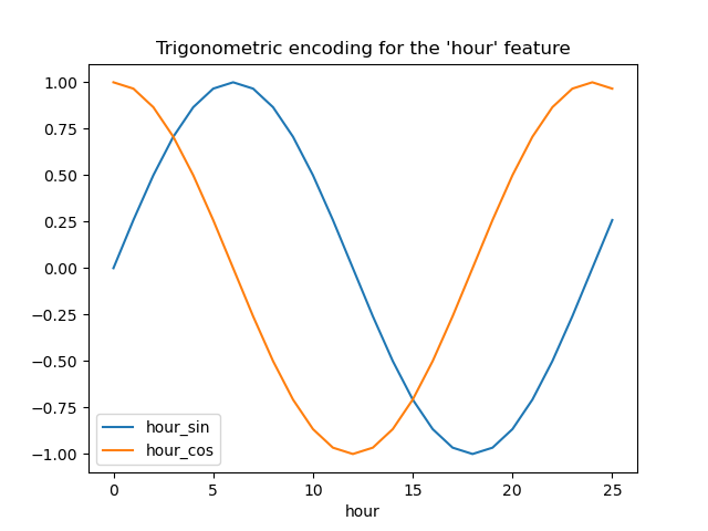
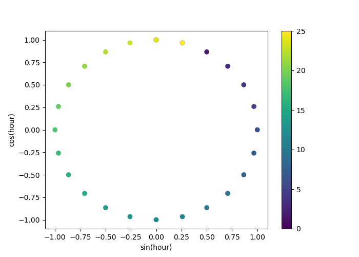
讓我們使用 2D 散點圖,以小時數作為顏色編碼,以更好地了解這種表示如何將一天中的 24 小時映射到 2D 空間,類似於某種 24 小時版本的類比時鐘。請注意,“第 25” 小時會因為正弦/餘弦表示的週期性而映射回第 1 小時。
fig, ax = plt.subplots(figsize=(7, 5))
sp = ax.scatter(hour_df["hour_sin"], hour_df["hour_cos"], c=hour_df["hour"])
ax.set(
    xlabel="sin(hour)",
    ylabel="cos(hour)",
)
_ = fig.colorbar(sp)
我們現在可以使用這種策略建立特徵提取管道
cyclic_cossin_transformer = ColumnTransformer(
    transformers=[
        ("categorical", one_hot_encoder, categorical_columns),
        ("month_sin", sin_transformer(12), ["month"]),
        ("month_cos", cos_transformer(12), ["month"]),
        ("weekday_sin", sin_transformer(7), ["weekday"]),
        ("weekday_cos", cos_transformer(7), ["weekday"]),
        ("hour_sin", sin_transformer(24), ["hour"]),
        ("hour_cos", cos_transformer(24), ["hour"]),
    ],
    remainder=MinMaxScaler(),
)
cyclic_cossin_linear_pipeline = make_pipeline(
    cyclic_cossin_transformer,
    RidgeCV(alphas=alphas),
)
evaluate(cyclic_cossin_linear_pipeline, X, y, cv=ts_cv)
Mean Absolute Error:     0.125 +/- 0.014
Root Mean Squared Error: 0.166 +/- 0.020
使用這種簡單的特徵工程,我們的線性迴歸模型的效能比使用原始序數時間特徵稍微好一點,但比使用獨熱編碼的時間特徵要差。我們將在本筆記本的最後分析造成這種令人失望的結果的可能原因。
週期性樣條特徵#
我們可以嘗試使用樣條轉換來替代週期性時間相關特徵的編碼,使用足夠多的樣條,因此與正弦/餘弦轉換相比,特徵擴展後的數量更多。
from sklearn.preprocessing import SplineTransformer


def periodic_spline_transformer(period, n_splines=None, degree=3):
    if n_splines is None:
        n_splines = period
    n_knots = n_splines + 1  # periodic and include_bias is True
    return SplineTransformer(
        degree=degree,
        n_knots=n_knots,
        knots=np.linspace(0, period, n_knots).reshape(n_knots, 1),
        extrapolation="periodic",
        include_bias=True,
    )
同樣,讓我們視覺化此特徵擴展對一些合成小時數據的影響,並稍微外推到 hour=23 之外
hour_df = pd.DataFrame(
    np.linspace(0, 26, 1000).reshape(-1, 1),
    columns=["hour"],
)
splines = periodic_spline_transformer(24, n_splines=12).fit_transform(hour_df)
splines_df = pd.DataFrame(
    splines,
    columns=[f"spline_{i}" for i in range(splines.shape[1])],
)
pd.concat([hour_df, splines_df], axis="columns").plot(x="hour", cmap=plt.cm.tab20b)
_ = plt.title("Periodic spline-based encoding for the 'hour' feature")
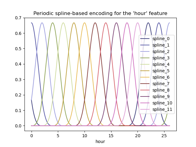
由於使用了 extrapolation="periodic" 參數,我們觀察到在午夜之後進行外推時,特徵編碼保持平滑。
我們現在可以使用這種替代的週期性特徵工程策略建立預測管道。
對於這些序數值,可以使用比離散級別更少的樣條。這使得基於樣條的編碼比獨熱編碼更有效,同時保留了大部分表達能力
cyclic_spline_transformer = ColumnTransformer(
    transformers=[
        ("categorical", one_hot_encoder, categorical_columns),
        ("cyclic_month", periodic_spline_transformer(12, n_splines=6), ["month"]),
        ("cyclic_weekday", periodic_spline_transformer(7, n_splines=3), ["weekday"]),
        ("cyclic_hour", periodic_spline_transformer(24, n_splines=12), ["hour"]),
    ],
    remainder=MinMaxScaler(),
)
cyclic_spline_linear_pipeline = make_pipeline(
    cyclic_spline_transformer,
    RidgeCV(alphas=alphas),
)
evaluate(cyclic_spline_linear_pipeline, X, y, cv=ts_cv)
Mean Absolute Error:     0.097 +/- 0.011
Root Mean Squared Error: 0.132 +/- 0.013
樣條特徵使線性模型能夠成功利用週期性時間相關特徵,並將誤差從最大需求的約 14% 降至約 10%,這與我們使用獨熱編碼特徵觀察到的情況類似。
線性模型預測中特徵影響的定性分析#
在這裡,我們想要視覺化特徵工程選擇對預測的時間相關形狀的影響。
為此,我們考慮一個任意的基於時間的分割,以比較在一系列保留的數據點上的預測。
naive_linear_pipeline.fit(X.iloc[train_0], y.iloc[train_0])
naive_linear_predictions = naive_linear_pipeline.predict(X.iloc[test_0])

one_hot_linear_pipeline.fit(X.iloc[train_0], y.iloc[train_0])
one_hot_linear_predictions = one_hot_linear_pipeline.predict(X.iloc[test_0])

cyclic_cossin_linear_pipeline.fit(X.iloc[train_0], y.iloc[train_0])
cyclic_cossin_linear_predictions = cyclic_cossin_linear_pipeline.predict(X.iloc[test_0])

cyclic_spline_linear_pipeline.fit(X.iloc[train_0], y.iloc[train_0])
cyclic_spline_linear_predictions = cyclic_spline_linear_pipeline.predict(X.iloc[test_0])
我們通過放大測試集的最後 96 小時(4 天)來視覺化這些預測,以獲得一些定性的見解
last_hours = slice(-96, None)
fig, ax = plt.subplots(figsize=(12, 4))
fig.suptitle("Predictions by linear models")
ax.plot(
    y.iloc[test_0].values[last_hours],
    "x-",
    alpha=0.2,
    label="Actual demand",
    color="black",
)
ax.plot(naive_linear_predictions[last_hours], "x-", label="Ordinal time features")
ax.plot(
    cyclic_cossin_linear_predictions[last_hours],
    "x-",
    label="Trigonometric time features",
)
ax.plot(
    cyclic_spline_linear_predictions[last_hours],
    "x-",
    label="Spline-based time features",
)
ax.plot(
    one_hot_linear_predictions[last_hours],
    "x-",
    label="One-hot time features",
)
_ = ax.legend()
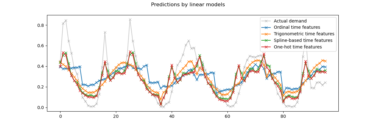
我們可以從上面的繪圖中得出以下結論
原始序數時間相關特徵是有問題的,因為它們沒有捕捉到自然的週期性:我們觀察到每天結束時當小時特徵從 23 返回到 0 時,預測會出現很大的跳躍。我們可以預期在每週或每年的結束時也會出現類似的偽影。
正如預期的那樣,三角函數特徵(正弦和餘弦)在午夜沒有這些不連續性,但線性迴歸模型未能利用這些特徵來正確建模日內變化。對自然週期使用更高諧波或額外的三角函數特徵(具有不同相位)可能會解決此問題。
基於週期性樣條的特徵一次解決了這兩個問題:它們通過使用 12 個樣條,使線性模型可以專注於特定小時,從而為線性模型提供了更多表達能力。此外,
extrapolation="periodic"選項強制執行hour=23和hour=0之間的平滑表示。獨熱編碼特徵的行為與基於週期性樣條的特徵類似,但更為尖銳:例如,它們可以更好地模擬工作日早晨的高峰,因為這個高峰持續時間短於一小時。但是,我們將在接下來看到,對線性模型來說可能是優勢的,對更具表達能力的模型來說不一定是優勢。
我們也可以比較每個特徵工程管道提取的特徵數量
naive_linear_pipeline[:-1].transform(X).shape
(17379, 19)
one_hot_linear_pipeline[:-1].transform(X).shape
(17379, 59)
cyclic_cossin_linear_pipeline[:-1].transform(X).shape
(17379, 22)
cyclic_spline_linear_pipeline[:-1].transform(X).shape
(17379, 37)
這證實了獨熱編碼和樣條編碼策略為時間表示創建了比替代方案更多的特徵,這反過來又為下游線性模型提供了更大的彈性(自由度),以避免欠擬合。
最後,我們觀察到,沒有一個線性模型可以近似真實的自行車租賃需求,特別是對於在工作日高峰時段非常尖銳的高峰,但在週末則平坦得多:基於樣條或獨熱編碼的最精確線性模型傾向於預測與通勤相關的自行車租賃高峰,即使在週末也是如此,並且低估了工作日期間與通勤相關的事件。
這些系統性的預測誤差揭示了一種欠擬合形式,可以用特徵之間缺乏交互作用項來解釋,例如“工作日”和從“小時”導出的特徵。此問題將在下一節中解決。
使用樣條和多項式特徵建模成對交互#
線性模型不會自動捕捉輸入特徵之間的交互作用效應。某些特徵是邊際非線性的,例如由 SplineTransformer(或獨熱編碼或分箱)構造的特徵,這沒有幫助。
但是,可以在粗粒度樣條編碼小時上使用 PolynomialFeatures 類,以明確建模 “workingday”/”hours” 交互作用,而不會引入太多新變數
from sklearn.pipeline import FeatureUnion
from sklearn.preprocessing import PolynomialFeatures

hour_workday_interaction = make_pipeline(
    ColumnTransformer(
        [
            ("cyclic_hour", periodic_spline_transformer(24, n_splines=8), ["hour"]),
            ("workingday", FunctionTransformer(lambda x: x == "True"), ["workingday"]),
        ]
    ),
    PolynomialFeatures(degree=2, interaction_only=True, include_bias=False),
)
然後,將這些特徵與先前基於樣條的管道中已計算的特徵組合在一起。我們可以觀察到,通過明確建模這種成對交互作用,效能得到了很好的提升
cyclic_spline_interactions_pipeline = make_pipeline(
    FeatureUnion(
        [
            ("marginal", cyclic_spline_transformer),
            ("interactions", hour_workday_interaction),
        ]
    ),
    RidgeCV(alphas=alphas),
)
evaluate(cyclic_spline_interactions_pipeline, X, y, cv=ts_cv)
Mean Absolute Error:     0.078 +/- 0.009
Root Mean Squared Error: 0.104 +/- 0.009
使用核心建模非線性特徵交互作用#
先前的分析強調了需要建模 "workingday" 和 "hours" 之間的交互作用。我們想要建模的另一個此類非線性交互作用的例子可能是降雨的影響,在工作日和週末和假日期間可能不同。
為了建模所有此類交互作用,我們可以在基於樣條的擴展之後,對所有邊緣特徵同時使用多項式擴展。但是,這會創建二次數量的特徵,這可能會導致過擬合和計算上的可處理性問題。
或者,我們可以使用 Nyström 方法來計算近似多項式核心擴展。讓我們嘗試後者
from sklearn.kernel_approximation import Nystroem

cyclic_spline_poly_pipeline = make_pipeline(
    cyclic_spline_transformer,
    Nystroem(kernel="poly", degree=2, n_components=300, random_state=0),
    RidgeCV(alphas=alphas),
)
evaluate(cyclic_spline_poly_pipeline, X, y, cv=ts_cv)
Mean Absolute Error:     0.053 +/- 0.002
Root Mean Squared Error: 0.076 +/- 0.004
我們觀察到,此模型的效能幾乎可以與梯度提升樹相媲美,平均誤差約為最大需求的 5%。
請注意,雖然此管道的最後一步是線性迴歸模型,但中間步驟(例如樣條特徵提取和 Nyström 核心近似)是高度非線性的。因此,複合管道比使用原始特徵的簡單線性迴歸模型更具表達能力。
為了完整起見,我們還評估了獨熱編碼和核心近似的組合
one_hot_poly_pipeline = make_pipeline(
    ColumnTransformer(
        transformers=[
            ("categorical", one_hot_encoder, categorical_columns),
            ("one_hot_time", one_hot_encoder, ["hour", "weekday", "month"]),
        ],
        remainder="passthrough",
    ),
    Nystroem(kernel="poly", degree=2, n_components=300, random_state=0),
    RidgeCV(alphas=alphas),
)
evaluate(one_hot_poly_pipeline, X, y, cv=ts_cv)
Mean Absolute Error:     0.082 +/- 0.006
Root Mean Squared Error: 0.111 +/- 0.011
雖然在使用線性模型時,獨熱編碼的特徵與基於樣條的特徵具有競爭力,但在使用非線性核心的低秩近似時,情況不再如此:這可以用樣條特徵更平滑來解釋,並允許核心近似找到更具表達能力的決策函數。
現在讓我們對核模型和梯度提升樹的預測進行定性觀察,它們應該能夠更好地模擬特徵之間的非線性交互作用。
gbrt.fit(X.iloc[train_0], y.iloc[train_0])
gbrt_predictions = gbrt.predict(X.iloc[test_0])

one_hot_poly_pipeline.fit(X.iloc[train_0], y.iloc[train_0])
one_hot_poly_predictions = one_hot_poly_pipeline.predict(X.iloc[test_0])

cyclic_spline_poly_pipeline.fit(X.iloc[train_0], y.iloc[train_0])
cyclic_spline_poly_predictions = cyclic_spline_poly_pipeline.predict(X.iloc[test_0])
再次,我們放大觀察測試集最後 4 天的數據。
last_hours = slice(-96, None)
fig, ax = plt.subplots(figsize=(12, 4))
fig.suptitle("Predictions by non-linear regression models")
ax.plot(
    y.iloc[test_0].values[last_hours],
    "x-",
    alpha=0.2,
    label="Actual demand",
    color="black",
)
ax.plot(
    gbrt_predictions[last_hours],
    "x-",
    label="Gradient Boosted Trees",
)
ax.plot(
    one_hot_poly_predictions[last_hours],
    "x-",
    label="One-hot + polynomial kernel",
)
ax.plot(
    cyclic_spline_poly_predictions[last_hours],
    "x-",
    label="Splines + polynomial kernel",
)
_ = ax.legend()
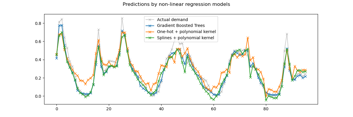
首先,請注意,樹模型可以自然地模擬非線性特徵交互作用,因為預設情況下,決策樹可以成長到超過 2 層的深度。
在這裡,我們可以觀察到,樣條特徵和非線性核的組合效果非常好,幾乎可以與梯度提升迴歸樹的準確度相媲美。
相反地,獨熱編碼的時間特徵在低秩核模型下的表現不佳。特別是,它們明顯高估了低需求時段的需求,程度比其他競爭模型更嚴重。
我們也觀察到,沒有任何模型可以成功預測工作日尖峰時段的一些租賃高峰。可能需要存取額外的特徵才能進一步提高預測的準確度。例如,如果能夠存取任何時間點的車隊地理分佈,或需要維修而無法使用的單車比例,可能會有所幫助。
最後,讓我們使用真實值 vs 預測需求散佈圖,更定量地觀察這三個模型的預測誤差。
from sklearn.metrics import PredictionErrorDisplay

fig, axes = plt.subplots(nrows=2, ncols=3, figsize=(13, 7), sharex=True, sharey="row")
fig.suptitle("Non-linear regression models", y=1.0)
predictions = [
    one_hot_poly_predictions,
    cyclic_spline_poly_predictions,
    gbrt_predictions,
]
labels = [
    "One hot +\npolynomial kernel",
    "Splines +\npolynomial kernel",
    "Gradient Boosted\nTrees",
]
plot_kinds = ["actual_vs_predicted", "residual_vs_predicted"]
for axis_idx, kind in enumerate(plot_kinds):
    for ax, pred, label in zip(axes[axis_idx], predictions, labels):
        disp = PredictionErrorDisplay.from_predictions(
            y_true=y.iloc[test_0],
            y_pred=pred,
            kind=kind,
            scatter_kwargs={"alpha": 0.3},
            ax=ax,
        )
        ax.set_xticks(np.linspace(0, 1, num=5))
        if axis_idx == 0:
            ax.set_yticks(np.linspace(0, 1, num=5))
            ax.legend(
                ["Best model", label],
                loc="upper center",
                bbox_to_anchor=(0.5, 1.3),
                ncol=2,
            )
        ax.set_aspect("equal", adjustable="box")
plt.show()
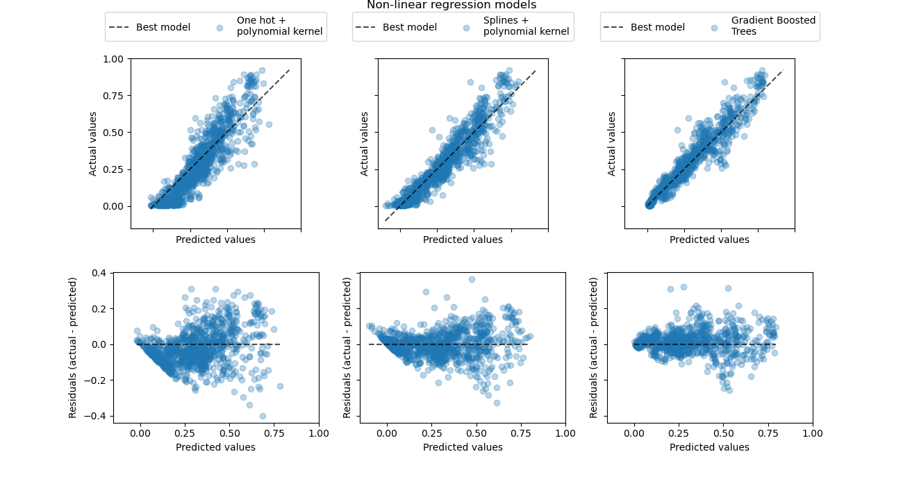
此視覺化呈現確認了我們在先前的圖表上得出的結論。
所有模型都低估了高需求事件(工作日尖峰時段),但梯度提升的低估程度較輕。梯度提升平均能很好地預測低需求事件,而獨熱編碼多項式迴歸管線似乎系統性地高估了該情況下的需求。總體而言,梯度提升樹的預測比核模型的預測更接近對角線。
總結#
我們注意到,透過使用更多的成分(更高秩的核近似),我們可以為核模型獲得稍微更好的結果,但代價是更長的擬合和預測時間。對於較大的 n_components 值,獨熱編碼特徵的性能甚至可以與樣條特徵相匹配。
Nystroem + RidgeCV 迴歸器也可以用具有一或兩個隱藏層的 MLPRegressor 取代,我們將獲得相當類似的結果。
本案例研究中使用的資料集是以每小時為基礎採樣的。然而,基於循環樣條的特徵可以非常有效地模擬一天內或一週內的時間,而且無需引入更多特徵,就可以使用更精細的時間解析度(例如,每分鐘而非每小時進行測量)。獨熱編碼時間表示則無法提供這種彈性。
最後,在本筆記本中,我們使用 RidgeCV,因為它在計算方面非常有效。然而,它將目標變數建模為具有恆定變異數的高斯隨機變數。對於正迴歸問題,使用 Poisson 或 Gamma 分佈可能更有意義。這可以使用 GridSearchCV(TweedieRegressor(power=2), param_grid({"alpha": alphas})) 而不是 RidgeCV 來實現。
腳本總執行時間: (0 分鐘 13.619 秒)
相關範例