注意
前往結尾以下載完整的範例程式碼。或透過 JupyterLite 或 Binder 在您的瀏覽器中執行此範例
聚類效能評估中針對機率調整#
這個筆記本探討均勻分佈的隨機標記對某些聚類評估指標行為的影響。為此,指標會使用固定數量的樣本計算,並作為估計器分配的聚類數量的函數。範例分為兩個實驗
第一個實驗具有固定的「真實標籤」(因此類別數量固定)和隨機「預測標籤」;
第二個實驗具有變化的「真實標籤」、隨機「預測標籤」。 「預測標籤」具有與「真實標籤」相同的類別和聚類數量。
# Authors: The scikit-learn developers
# SPDX-License-Identifier: BSD-3-Clause
定義要評估的指標列表#
聚類演算法基本上是無監督學習方法。然而,由於我們在此範例中為合成聚類分配了類別標籤,因此可以使用利用此「監督」真實資訊的評估指標,來量化所得聚類的品質。此類指標的範例如下
V-量度,完整性和同質性的調和平均值;
Rand 指數,它測量資料點對根據聚類演算法的結果和真實類別分配進行一致分組的頻率;
調整的 Rand 指數 (ARI),一種經過機率調整的 Rand 指數,使得隨機聚類分配的期望 ARI 為 0.0;
互資訊 (MI) 是一種資訊理論度量,量化兩個標記的依賴程度。請注意,完美標記的 MI 最大值取決於聚類和樣本的數量;
正規化互資訊 (NMI),在大量資料點的限制下,定義在 0(沒有互資訊)和 1(完美匹配標籤分配,直到標籤排列)之間的互資訊。它沒有針對機率進行調整:那麼如果聚類資料點的數量不夠大,則隨機標記的 MI 或 NMI 的預期值可能會顯著不為零;
調整的互資訊 (AMI),一種經過機率調整的互資訊。與 ARI 類似,隨機聚類分配的期望 AMI 為 0.0。
如需更多資訊,請參閱 聚類效能評估 模組。
from sklearn import metrics

score_funcs = [
    ("V-measure", metrics.v_measure_score),
    ("Rand index", metrics.rand_score),
    ("ARI", metrics.adjusted_rand_score),
    ("MI", metrics.mutual_info_score),
    ("NMI", metrics.normalized_mutual_info_score),
    ("AMI", metrics.adjusted_mutual_info_score),
]
第一個實驗:固定的真實標籤和不斷增加的聚類數量#
我們首先定義一個建立均勻分佈隨機標記的函數。
import numpy as np

rng = np.random.RandomState(0)


def random_labels(n_samples, n_classes):
    return rng.randint(low=0, high=n_classes, size=n_samples)
另一個函數將使用 random_labels 函數建立一組固定的真實標籤 (labels_a),分佈在 n_classes 中,然後對幾組隨機「預測」標籤 (labels_b) 進行評分,以評估在給定 n_clusters 下,給定指標的變異性。
def fixed_classes_uniform_labelings_scores(
    score_func, n_samples, n_clusters_range, n_classes, n_runs=5
):
    scores = np.zeros((len(n_clusters_range), n_runs))
    labels_a = random_labels(n_samples=n_samples, n_classes=n_classes)

    for i, n_clusters in enumerate(n_clusters_range):
        for j in range(n_runs):
            labels_b = random_labels(n_samples=n_samples, n_classes=n_clusters)
            scores[i, j] = score_func(labels_a, labels_b)
    return scores
在第一個範例中,我們將類別數量(聚類的真實數量)設定為 n_classes=10。聚類數量在 n_clusters_range 提供的值範圍內變化。
import matplotlib.pyplot as plt
import seaborn as sns

n_samples = 1000
n_classes = 10
n_clusters_range = np.linspace(2, 100, 10).astype(int)
plots = []
names = []

sns.color_palette("colorblind")
plt.figure(1)

for marker, (score_name, score_func) in zip("d^vx.,", score_funcs):
    scores = fixed_classes_uniform_labelings_scores(
        score_func, n_samples, n_clusters_range, n_classes=n_classes
    )
    plots.append(
        plt.errorbar(
            n_clusters_range,
            scores.mean(axis=1),
            scores.std(axis=1),
            alpha=0.8,
            linewidth=1,
            marker=marker,
        )[0]
    )
    names.append(score_name)

plt.title(
    "Clustering measures for random uniform labeling\n"
    f"against reference assignment with {n_classes} classes"
)
plt.xlabel(f"Number of clusters (Number of samples is fixed to {n_samples})")
plt.ylabel("Score value")
plt.ylim(bottom=-0.05, top=1.05)
plt.legend(plots, names, bbox_to_anchor=(0.5, 0.5))
plt.show()
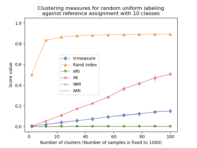
Rand 指數在 n_clusters > n_classes 時飽和。其他未調整的度量(例如 V 量度)顯示聚類數量和樣本數量之間存在線性相依性。
針對機率調整的度量(例如 ARI 和 AMI)顯示一些隨機變化,這些變化圍繞平均分數 0.0 為中心,獨立於樣本和聚類的數量。
第二個實驗:變化的類別和聚類數量#
在本節中,我們定義一個類似的函數,使用多個指標對 2 個均勻分佈的隨機標記進行評分。在這種情況下,類別數量和分配的聚類數量與 n_clusters_range 中每個可能的值相匹配。
def uniform_labelings_scores(score_func, n_samples, n_clusters_range, n_runs=5):
    scores = np.zeros((len(n_clusters_range), n_runs))

    for i, n_clusters in enumerate(n_clusters_range):
        for j in range(n_runs):
            labels_a = random_labels(n_samples=n_samples, n_classes=n_clusters)
            labels_b = random_labels(n_samples=n_samples, n_classes=n_clusters)
            scores[i, j] = score_func(labels_a, labels_b)
    return scores
在這種情況下,我們使用 n_samples=100 來顯示聚類數量與樣本數量相似或相等的效果。
n_samples = 100
n_clusters_range = np.linspace(2, n_samples, 10).astype(int)

plt.figure(2)

plots = []
names = []

for marker, (score_name, score_func) in zip("d^vx.,", score_funcs):
    scores = uniform_labelings_scores(score_func, n_samples, n_clusters_range)
    plots.append(
        plt.errorbar(
            n_clusters_range,
            np.median(scores, axis=1),
            scores.std(axis=1),
            alpha=0.8,
            linewidth=2,
            marker=marker,
        )[0]
    )
    names.append(score_name)

plt.title(
    "Clustering measures for 2 random uniform labelings\nwith equal number of clusters"
)
plt.xlabel(f"Number of clusters (Number of samples is fixed to {n_samples})")
plt.ylabel("Score value")
plt.legend(plots, names)
plt.ylim(bottom=-0.05, top=1.05)
plt.show()
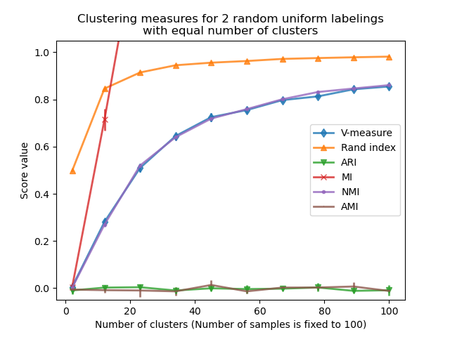
我們觀察到與第一個實驗類似的結果:針對機率調整的指標始終保持在零附近,而其他指標隨著更精細的標記而變大。隨著聚類數量越來越接近用於計算度量的樣本總數,隨機標記的平均 V 量度顯著增加。此外,原始互資訊不受上限限制,其規模取決於聚類問題的維度和真實類別的基數。這就是為什麼曲線超出圖表範圍的原因。
因此,只有調整後的度量才能安全地用作共識索引,以評估聚類演算法在數據集多個重疊子樣本上針對給定的 k 值的平均穩定性。
因此,未調整的聚類評估指標可能會產生誤導,因為它們會為精細的標記輸出較大的值,人們可能會認為標記已捕獲有意義的組,而它們可能是完全隨機的。特別是,不應使用此類未調整的指標來比較輸出不同聚類數量的不同聚類演算法的結果。
腳本的總運行時間: (0 分鐘 0.987 秒)
相關範例