不同核函數的高斯過程的先驗與後驗說明#

此範例說明具有不同核函數的GaussianProcessRegressor的高斯過程的先驗和後驗。顯示先驗和後驗分佈的平均值、標準差和 5 個樣本。

在此，我們只給出一些說明。若要進一步了解核函數的公式，請參閱使用者指南。

# Authors: The scikit-learn developers
# SPDX-License-Identifier: BSD-3-Clause

輔助函數#

在介紹可供高斯過程使用的每個核函數之前，我們將定義一個輔助函數，讓我們可以繪製從高斯過程提取的樣本。

此函數將取得GaussianProcessRegressor模型，並從高斯過程提取樣本。如果模型尚未擬合，則樣本是從先驗分佈中提取，而在模型擬合後，樣本是從後驗分佈中提取。

import matplotlib.pyplot as plt
import numpy as np


def plot_gpr_samples(gpr_model, n_samples, ax):
    """Plot samples drawn from the Gaussian process model.

    If the Gaussian process model is not trained then the drawn samples are
    drawn from the prior distribution. Otherwise, the samples are drawn from
    the posterior distribution. Be aware that a sample here corresponds to a
    function.

    Parameters
    ----------
    gpr_model : `GaussianProcessRegressor`
        A :class:`~sklearn.gaussian_process.GaussianProcessRegressor` model.
    n_samples : int
        The number of samples to draw from the Gaussian process distribution.
    ax : matplotlib axis
        The matplotlib axis where to plot the samples.
    """
    x = np.linspace(0, 5, 100)
    X = x.reshape(-1, 1)

    y_mean, y_std = gpr_model.predict(X, return_std=True)
    y_samples = gpr_model.sample_y(X, n_samples)

    for idx, single_prior in enumerate(y_samples.T):
        ax.plot(
            x,
            single_prior,
            linestyle="--",
            alpha=0.7,
            label=f"Sampled function #{idx + 1}",
        )
    ax.plot(x, y_mean, color="black", label="Mean")
    ax.fill_between(
        x,
        y_mean - y_std,
        y_mean + y_std,
        alpha=0.1,
        color="black",
        label=r"$\pm$ 1 std. dev.",
    )
    ax.set_xlabel("x")
    ax.set_ylabel("y")
    ax.set_ylim([-3, 3])

資料集和高斯過程生成#

我們將建立一個訓練資料集，我們將在不同的章節中使用它。

rng = np.random.RandomState(4)
X_train = rng.uniform(0, 5, 10).reshape(-1, 1)
y_train = np.sin((X_train[:, 0] - 2.5) ** 2)
n_samples = 5

核函數食譜#

在本節中，我們說明一些從具有不同核函數的高斯過程的先驗和後驗分佈中提取的樣本。

徑向基底函數核函數#

from sklearn.gaussian_process import GaussianProcessRegressor
from sklearn.gaussian_process.kernels import RBF

kernel = 1.0 * RBF(length_scale=1.0, length_scale_bounds=(1e-1, 10.0))
gpr = GaussianProcessRegressor(kernel=kernel, random_state=0)

fig, axs = plt.subplots(nrows=2, sharex=True, sharey=True, figsize=(10, 8))

# plot prior
plot_gpr_samples(gpr, n_samples=n_samples, ax=axs[0])
axs[0].set_title("Samples from prior distribution")

# plot posterior
gpr.fit(X_train, y_train)
plot_gpr_samples(gpr, n_samples=n_samples, ax=axs[1])
axs[1].scatter(X_train[:, 0], y_train, color="red", zorder=10, label="Observations")
axs[1].legend(bbox_to_anchor=(1.05, 1.5), loc="upper left")
axs[1].set_title("Samples from posterior distribution")

fig.suptitle("Radial Basis Function kernel", fontsize=18)
plt.tight_layout()

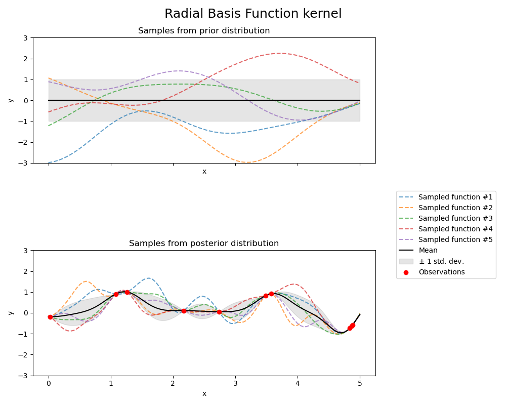
Radial Basis Function kernel, Samples from prior distribution, Samples from posterior distribution

print(f"Kernel parameters before fit:\n{kernel})")
print(
    f"Kernel parameters after fit: \n{gpr.kernel_} \n"
    f"Log-likelihood: {gpr.log_marginal_likelihood(gpr.kernel_.theta):.3f}"
)

Kernel parameters before fit:
1**2 * RBF(length_scale=1))
Kernel parameters after fit:
0.594**2 * RBF(length_scale=0.279)
Log-likelihood: -0.067

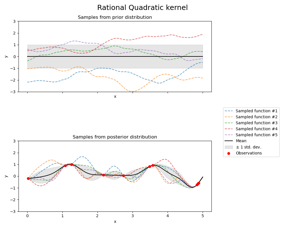
有理二次核函數#

from sklearn.gaussian_process.kernels import RationalQuadratic

kernel = 1.0 * RationalQuadratic(length_scale=1.0, alpha=0.1, alpha_bounds=(1e-5, 1e15))
gpr = GaussianProcessRegressor(kernel=kernel, random_state=0)

fig, axs = plt.subplots(nrows=2, sharex=True, sharey=True, figsize=(10, 8))

# plot prior
plot_gpr_samples(gpr, n_samples=n_samples, ax=axs[0])
axs[0].set_title("Samples from prior distribution")

# plot posterior
gpr.fit(X_train, y_train)
plot_gpr_samples(gpr, n_samples=n_samples, ax=axs[1])
axs[1].scatter(X_train[:, 0], y_train, color="red", zorder=10, label="Observations")
axs[1].legend(bbox_to_anchor=(1.05, 1.5), loc="upper left")
axs[1].set_title("Samples from posterior distribution")

fig.suptitle("Rational Quadratic kernel", fontsize=18)
plt.tight_layout()

Rational Quadratic kernel, Samples from prior distribution, Samples from posterior distribution

/home/circleci/project/sklearn/gaussian_process/_gpr.py:523: RuntimeWarning:

covariance is not symmetric positive-semidefinite.

print(f"Kernel parameters before fit:\n{kernel})")
print(
    f"Kernel parameters after fit: \n{gpr.kernel_} \n"
    f"Log-likelihood: {gpr.log_marginal_likelihood(gpr.kernel_.theta):.3f}"
)

Kernel parameters before fit:
1**2 * RationalQuadratic(alpha=0.1, length_scale=1))
Kernel parameters after fit:
0.594**2 * RationalQuadratic(alpha=6.69e+08, length_scale=0.279)
Log-likelihood: -0.067

指數正弦平方核函數#

from sklearn.gaussian_process.kernels import ExpSineSquared

kernel = 1.0 * ExpSineSquared(
    length_scale=1.0,
    periodicity=3.0,
    length_scale_bounds=(0.1, 10.0),
    periodicity_bounds=(1.0, 10.0),
)
gpr = GaussianProcessRegressor(kernel=kernel, random_state=0)

fig, axs = plt.subplots(nrows=2, sharex=True, sharey=True, figsize=(10, 8))

# plot prior
plot_gpr_samples(gpr, n_samples=n_samples, ax=axs[0])
axs[0].set_title("Samples from prior distribution")

# plot posterior
gpr.fit(X_train, y_train)
plot_gpr_samples(gpr, n_samples=n_samples, ax=axs[1])
axs[1].scatter(X_train[:, 0], y_train, color="red", zorder=10, label="Observations")
axs[1].legend(bbox_to_anchor=(1.05, 1.5), loc="upper left")
axs[1].set_title("Samples from posterior distribution")

fig.suptitle("Exp-Sine-Squared kernel", fontsize=18)
plt.tight_layout()

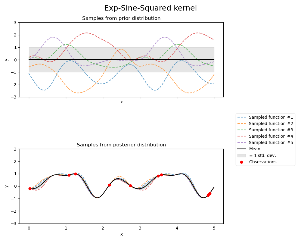
Exp-Sine-Squared kernel, Samples from prior distribution, Samples from posterior distribution

print(f"Kernel parameters before fit:\n{kernel})")
print(
    f"Kernel parameters after fit: \n{gpr.kernel_} \n"
    f"Log-likelihood: {gpr.log_marginal_likelihood(gpr.kernel_.theta):.3f}"
)

Kernel parameters before fit:
1**2 * ExpSineSquared(length_scale=1, periodicity=3))
Kernel parameters after fit:
0.799**2 * ExpSineSquared(length_scale=0.791, periodicity=2.87)
Log-likelihood: 3.394

點積核函數#

from sklearn.gaussian_process.kernels import ConstantKernel, DotProduct

kernel = ConstantKernel(0.1, (0.01, 10.0)) * (
    DotProduct(sigma_0=1.0, sigma_0_bounds=(0.1, 10.0)) ** 2
)
gpr = GaussianProcessRegressor(kernel=kernel, random_state=0, normalize_y=True)

fig, axs = plt.subplots(nrows=2, sharex=True, sharey=True, figsize=(10, 8))

# plot prior
plot_gpr_samples(gpr, n_samples=n_samples, ax=axs[0])
axs[0].set_title("Samples from prior distribution")

# plot posterior
gpr.fit(X_train, y_train)
plot_gpr_samples(gpr, n_samples=n_samples, ax=axs[1])
axs[1].scatter(X_train[:, 0], y_train, color="red", zorder=10, label="Observations")
axs[1].legend(bbox_to_anchor=(1.05, 1.5), loc="upper left")
axs[1].set_title("Samples from posterior distribution")

fig.suptitle("Dot-product kernel", fontsize=18)
plt.tight_layout()

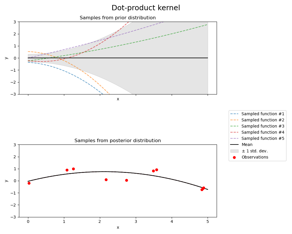
Dot-product kernel, Samples from prior distribution, Samples from posterior distribution

print(f"Kernel parameters before fit:\n{kernel})")
print(
    f"Kernel parameters after fit: \n{gpr.kernel_} \n"
    f"Log-likelihood: {gpr.log_marginal_likelihood(gpr.kernel_.theta):.3f}"
)

Kernel parameters before fit:
0.316**2 * DotProduct(sigma_0=1) ** 2)
Kernel parameters after fit:
0.697**2 * DotProduct(sigma_0=0.454) ** 2
Log-likelihood: -18108182014.707

Matérn 核函數#

from sklearn.gaussian_process.kernels import Matern

kernel = 1.0 * Matern(length_scale=1.0, length_scale_bounds=(1e-1, 10.0), nu=1.5)
gpr = GaussianProcessRegressor(kernel=kernel, random_state=0)

fig, axs = plt.subplots(nrows=2, sharex=True, sharey=True, figsize=(10, 8))

# plot prior
plot_gpr_samples(gpr, n_samples=n_samples, ax=axs[0])
axs[0].set_title("Samples from prior distribution")

# plot posterior
gpr.fit(X_train, y_train)
plot_gpr_samples(gpr, n_samples=n_samples, ax=axs[1])
axs[1].scatter(X_train[:, 0], y_train, color="red", zorder=10, label="Observations")
axs[1].legend(bbox_to_anchor=(1.05, 1.5), loc="upper left")
axs[1].set_title("Samples from posterior distribution")

fig.suptitle("Matérn kernel", fontsize=18)
plt.tight_layout()

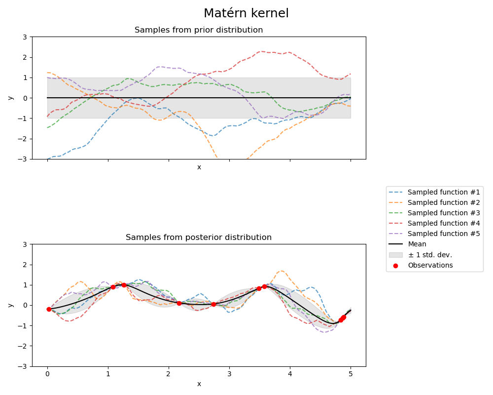
Matérn kernel, Samples from prior distribution, Samples from posterior distribution

print(f"Kernel parameters before fit:\n{kernel})")
print(
    f"Kernel parameters after fit: \n{gpr.kernel_} \n"
    f"Log-likelihood: {gpr.log_marginal_likelihood(gpr.kernel_.theta):.3f}"
)

Kernel parameters before fit:
1**2 * Matern(length_scale=1, nu=1.5))
Kernel parameters after fit:
0.609**2 * Matern(length_scale=0.484, nu=1.5)
Log-likelihood: -1.185

腳本的總執行時間： (0 分鐘 1.851 秒)