注意
前往結尾以下載完整的範例程式碼。或透過 JupyterLite 或 Binder 在您的瀏覽器中執行此範例
快取最近鄰#
此範例示範如何在 KNeighborsClassifier 中使用 k 個最近鄰之前預先計算它們。KNeighborsClassifier 可以在內部計算最近鄰,但預先計算它們可以有幾個好處,例如更精細的參數控制、快取以供多次使用或自訂實作。
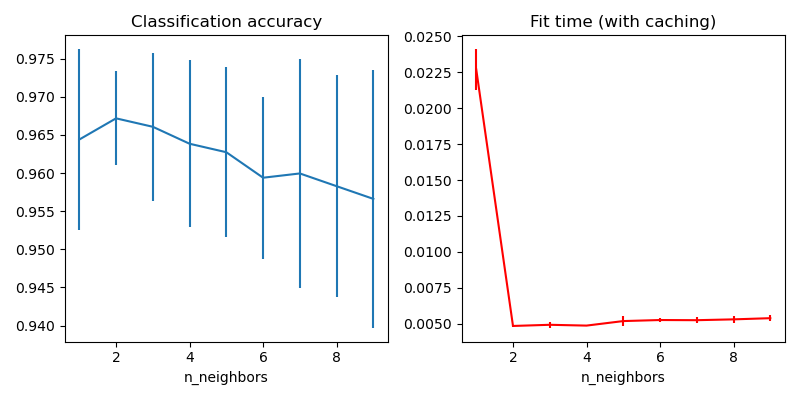
在此,我們使用管道的快取屬性來快取 KNeighborsClassifier 的多個擬合之間的最近鄰圖。第一次呼叫速度較慢,因為它會計算鄰居圖,而後續呼叫速度較快,因為它們不需要重新計算圖。由於資料集很小,這裡的持續時間很短,但當資料集變大或要搜尋的參數網格很大時,增益可能會更大。
# Authors: The scikit-learn developers
# SPDX-License-Identifier: BSD-3-Clause

from tempfile import TemporaryDirectory

import matplotlib.pyplot as plt

from sklearn.datasets import load_digits
from sklearn.model_selection import GridSearchCV
from sklearn.neighbors import KNeighborsClassifier, KNeighborsTransformer
from sklearn.pipeline import Pipeline

X, y = load_digits(return_X_y=True)
n_neighbors_list = [1, 2, 3, 4, 5, 6, 7, 8, 9]

# The transformer computes the nearest neighbors graph using the maximum number
# of neighbors necessary in the grid search. The classifier model filters the
# nearest neighbors graph as required by its own n_neighbors parameter.
graph_model = KNeighborsTransformer(n_neighbors=max(n_neighbors_list), mode="distance")
classifier_model = KNeighborsClassifier(metric="precomputed")

# Note that we give `memory` a directory to cache the graph computation
# that will be used several times when tuning the hyperparameters of the
# classifier.
with TemporaryDirectory(prefix="sklearn_graph_cache_") as tmpdir:
    full_model = Pipeline(
        steps=[("graph", graph_model), ("classifier", classifier_model)], memory=tmpdir
    )

    param_grid = {"classifier__n_neighbors": n_neighbors_list}
    grid_model = GridSearchCV(full_model, param_grid)
    grid_model.fit(X, y)

# Plot the results of the grid search.
fig, axes = plt.subplots(1, 2, figsize=(8, 4))
axes[0].errorbar(
    x=n_neighbors_list,
    y=grid_model.cv_results_["mean_test_score"],
    yerr=grid_model.cv_results_["std_test_score"],
)
axes[0].set(xlabel="n_neighbors", title="Classification accuracy")
axes[1].errorbar(
    x=n_neighbors_list,
    y=grid_model.cv_results_["mean_fit_time"],
    yerr=grid_model.cv_results_["std_fit_time"],
    color="r",
)
axes[1].set(xlabel="n_neighbors", title="Fit time (with caching)")
fig.tight_layout()
plt.show()
腳本總執行時間: (0 分鐘 1.454 秒)
相關範例