比較交叉分解方法#

各種交叉分解演算法的簡單用法

PLSCanonical
PLSRegression，具有多變數響應，又名 PLS2
PLSRegression，具有單變數響應，又名 PLS1
CCA

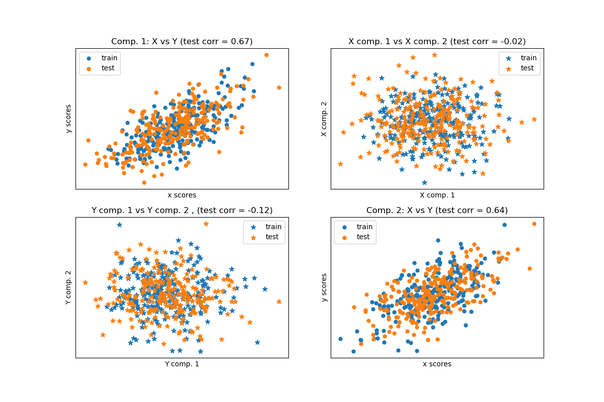
給定 2 個多變數共變二維資料集 X 和 Y，PLS 會提取「共變的方向」，即每個資料集的成分，這些成分解釋了兩個資料集之間最多的共享變異數。這在散佈圖矩陣顯示中很明顯：資料集 X 和資料集 Y 中的成分 1 最大相關（點位於第一條對角線附近）。這也適用於兩個資料集中的成分 2，但是，不同成分的跨資料集相關性較弱：點雲非常呈球形。

# Authors: The scikit-learn developers
# SPDX-License-Identifier: BSD-3-Clause

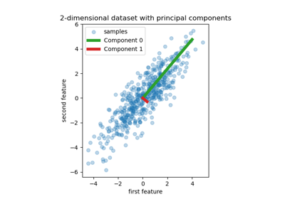
基於資料集的潛在變數模型#

import numpy as np

n = 500
# 2 latents vars:
l1 = np.random.normal(size=n)
l2 = np.random.normal(size=n)

latents = np.array([l1, l1, l2, l2]).T
X = latents + np.random.normal(size=4 * n).reshape((n, 4))
Y = latents + np.random.normal(size=4 * n).reshape((n, 4))

X_train = X[: n // 2]
Y_train = Y[: n // 2]
X_test = X[n // 2 :]
Y_test = Y[n // 2 :]

print("Corr(X)")
print(np.round(np.corrcoef(X.T), 2))
print("Corr(Y)")
print(np.round(np.corrcoef(Y.T), 2))

Corr(X)
[[ 1.    0.45 -0.04  0.  ]
 [ 0.45  1.   -0.1  -0.02]
 [-0.04 -0.1   1.    0.42]
 [ 0.   -0.02  0.42  1.  ]]
Corr(Y)
[[ 1.    0.48 -0.12 -0.05]
 [ 0.48  1.    0.07  0.04]
 [-0.12  0.07  1.    0.5 ]
 [-0.05  0.04  0.5   1.  ]]

標準（對稱）PLS#

轉換資料#

from sklearn.cross_decomposition import PLSCanonical

plsca = PLSCanonical(n_components=2)
plsca.fit(X_train, Y_train)
X_train_r, Y_train_r = plsca.transform(X_train, Y_train)
X_test_r, Y_test_r = plsca.transform(X_test, Y_test)

分數的散佈圖#

import matplotlib.pyplot as plt

# On diagonal plot X vs Y scores on each components
plt.figure(figsize=(12, 8))
plt.subplot(221)
plt.scatter(X_train_r[:, 0], Y_train_r[:, 0], label="train", marker="o", s=25)
plt.scatter(X_test_r[:, 0], Y_test_r[:, 0], label="test", marker="o", s=25)
plt.xlabel("x scores")
plt.ylabel("y scores")
plt.title(
    "Comp. 1: X vs Y (test corr = %.2f)"
    % np.corrcoef(X_test_r[:, 0], Y_test_r[:, 0])[0, 1]
)
plt.xticks(())
plt.yticks(())
plt.legend(loc="best")

plt.subplot(224)
plt.scatter(X_train_r[:, 1], Y_train_r[:, 1], label="train", marker="o", s=25)
plt.scatter(X_test_r[:, 1], Y_test_r[:, 1], label="test", marker="o", s=25)
plt.xlabel("x scores")
plt.ylabel("y scores")
plt.title(
    "Comp. 2: X vs Y (test corr = %.2f)"
    % np.corrcoef(X_test_r[:, 1], Y_test_r[:, 1])[0, 1]
)
plt.xticks(())
plt.yticks(())
plt.legend(loc="best")

# Off diagonal plot components 1 vs 2 for X and Y
plt.subplot(222)
plt.scatter(X_train_r[:, 0], X_train_r[:, 1], label="train", marker="*", s=50)
plt.scatter(X_test_r[:, 0], X_test_r[:, 1], label="test", marker="*", s=50)
plt.xlabel("X comp. 1")
plt.ylabel("X comp. 2")
plt.title(
    "X comp. 1 vs X comp. 2 (test corr = %.2f)"
    % np.corrcoef(X_test_r[:, 0], X_test_r[:, 1])[0, 1]
)
plt.legend(loc="best")
plt.xticks(())
plt.yticks(())

plt.subplot(223)
plt.scatter(Y_train_r[:, 0], Y_train_r[:, 1], label="train", marker="*", s=50)
plt.scatter(Y_test_r[:, 0], Y_test_r[:, 1], label="test", marker="*", s=50)
plt.xlabel("Y comp. 1")
plt.ylabel("Y comp. 2")
plt.title(
    "Y comp. 1 vs Y comp. 2 , (test corr = %.2f)"
    % np.corrcoef(Y_test_r[:, 0], Y_test_r[:, 1])[0, 1]
)
plt.legend(loc="best")
plt.xticks(())
plt.yticks(())
plt.show()

Comp. 1: X vs Y (test corr = 0.67), Comp. 2: X vs Y (test corr = 0.64), X comp. 1 vs X comp. 2 (test corr = -0.02), Y comp. 1 vs Y comp. 2 , (test corr = -0.12)

PLS 迴歸，具有多變數響應，又名 PLS2#

from sklearn.cross_decomposition import PLSRegression

n = 1000
q = 3
p = 10
X = np.random.normal(size=n * p).reshape((n, p))
B = np.array([[1, 2] + [0] * (p - 2)] * q).T
# each Yj = 1*X1 + 2*X2 + noize
Y = np.dot(X, B) + np.random.normal(size=n * q).reshape((n, q)) + 5

pls2 = PLSRegression(n_components=3)
pls2.fit(X, Y)
print("True B (such that: Y = XB + Err)")
print(B)
# compare pls2.coef_ with B
print("Estimated B")
print(np.round(pls2.coef_, 1))
pls2.predict(X)

True B (such that: Y = XB + Err)
[[1 1 1]
 [2 2 2]
 [0 0 0]
 [0 0 0]
 [0 0 0]
 [0 0 0]
 [0 0 0]
 [0 0 0]
 [0 0 0]
 [0 0 0]]
Estimated B
[[ 1.   2.   0.  -0.  -0.   0.   0.  -0.   0.   0. ]
 [ 1.   1.9  0.  -0.  -0.   0.1  0.   0.   0.   0. ]
 [ 1.   2.1 -0.   0.  -0.   0.   0.   0.   0.  -0. ]]

array([[4.11693539, 4.19803308, 4.12190903],
       [8.77322639, 8.77777215, 9.04995982],
       [5.34990341, 5.37257991, 5.27597342],
       ...,
       [5.95433992, 5.9403917 , 6.02818216],
       [5.06880943, 5.08604995, 5.05216586],
       [9.72295655, 9.70432034, 9.79769376]])

PLS 迴歸，具有單變數響應，又名 PLS1#

n = 1000
p = 10
X = np.random.normal(size=n * p).reshape((n, p))
y = X[:, 0] + 2 * X[:, 1] + np.random.normal(size=n * 1) + 5
pls1 = PLSRegression(n_components=3)
pls1.fit(X, y)
# note that the number of components exceeds 1 (the dimension of y)
print("Estimated betas")
print(np.round(pls1.coef_, 1))

Estimated betas
[[ 1.   2.  -0.1  0.  -0.  -0.  -0.   0.   0.  -0.1]]

CCA（具有對稱收縮的 PLS 模式 B）#

from sklearn.cross_decomposition import CCA

cca = CCA(n_components=2)
cca.fit(X_train, Y_train)
X_train_r, Y_train_r = cca.transform(X_train, Y_train)
X_test_r, Y_test_r = cca.transform(X_test, Y_test)