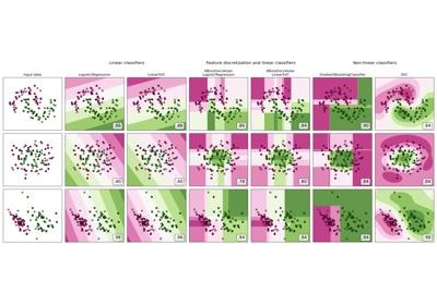
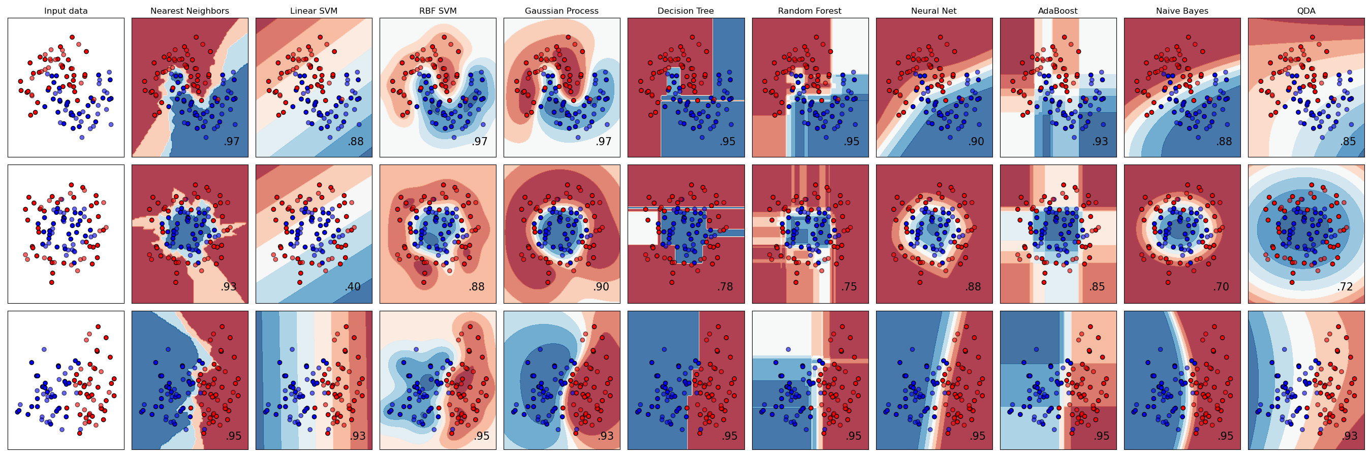
分類器比較#

在 scikit-learn 中對合成數據集進行幾個分類器的比較。此範例的目的是說明不同分類器的決策邊界的本質。這應該以懷疑的態度看待，因為這些範例傳達的直覺不一定適用於真實數據集。

特別是在高維空間中，數據更容易線性分離，而樸素貝葉斯和線性 SVM 等分類器的簡單性可能比其他分類器實現更好的泛化。

這些圖以實心顏色顯示訓練點，並以半透明顯示測試點。右下角顯示測試集上的分類準確度。

Input data, Nearest Neighbors, Linear SVM, RBF SVM, Gaussian Process, Decision Tree, Random Forest, Neural Net, AdaBoost, Naive Bayes, QDA

# Authors: The scikit-learn developers
# SPDX-License-Identifier: BSD-3-Clause

import matplotlib.pyplot as plt
import numpy as np
from matplotlib.colors import ListedColormap

from sklearn.datasets import make_circles, make_classification, make_moons
from sklearn.discriminant_analysis import QuadraticDiscriminantAnalysis
from sklearn.ensemble import AdaBoostClassifier, RandomForestClassifier
from sklearn.gaussian_process import GaussianProcessClassifier
from sklearn.gaussian_process.kernels import RBF
from sklearn.inspection import DecisionBoundaryDisplay
from sklearn.model_selection import train_test_split
from sklearn.naive_bayes import GaussianNB
from sklearn.neighbors import KNeighborsClassifier
from sklearn.neural_network import MLPClassifier
from sklearn.pipeline import make_pipeline
from sklearn.preprocessing import StandardScaler
from sklearn.svm import SVC
from sklearn.tree import DecisionTreeClassifier

names = [
    "Nearest Neighbors",
    "Linear SVM",
    "RBF SVM",
    "Gaussian Process",
    "Decision Tree",
    "Random Forest",
    "Neural Net",
    "AdaBoost",
    "Naive Bayes",
    "QDA",
]

classifiers = [
    KNeighborsClassifier(3),
    SVC(kernel="linear", C=0.025, random_state=42),
    SVC(gamma=2, C=1, random_state=42),
    GaussianProcessClassifier(1.0 * RBF(1.0), random_state=42),
    DecisionTreeClassifier(max_depth=5, random_state=42),
    RandomForestClassifier(
        max_depth=5, n_estimators=10, max_features=1, random_state=42
    ),
    MLPClassifier(alpha=1, max_iter=1000, random_state=42),
    AdaBoostClassifier(random_state=42),
    GaussianNB(),
    QuadraticDiscriminantAnalysis(),
]

X, y = make_classification(
    n_features=2, n_redundant=0, n_informative=2, random_state=1, n_clusters_per_class=1
)
rng = np.random.RandomState(2)
X += 2 * rng.uniform(size=X.shape)
linearly_separable = (X, y)

datasets = [
    make_moons(noise=0.3, random_state=0),
    make_circles(noise=0.2, factor=0.5, random_state=1),
    linearly_separable,
]

figure = plt.figure(figsize=(27, 9))
i = 1
# iterate over datasets
for ds_cnt, ds in enumerate(datasets):
    # preprocess dataset, split into training and test part
    X, y = ds
    X_train, X_test, y_train, y_test = train_test_split(
        X, y, test_size=0.4, random_state=42
    )

    x_min, x_max = X[:, 0].min() - 0.5, X[:, 0].max() + 0.5
    y_min, y_max = X[:, 1].min() - 0.5, X[:, 1].max() + 0.5

    # just plot the dataset first
    cm = plt.cm.RdBu
    cm_bright = ListedColormap(["#FF0000", "#0000FF"])
    ax = plt.subplot(len(datasets), len(classifiers) + 1, i)
    if ds_cnt == 0:
        ax.set_title("Input data")
    # Plot the training points
    ax.scatter(X_train[:, 0], X_train[:, 1], c=y_train, cmap=cm_bright, edgecolors="k")
    # Plot the testing points
    ax.scatter(
        X_test[:, 0], X_test[:, 1], c=y_test, cmap=cm_bright, alpha=0.6, edgecolors="k"
    )
    ax.set_xlim(x_min, x_max)
    ax.set_ylim(y_min, y_max)
    ax.set_xticks(())
    ax.set_yticks(())
    i += 1

    # iterate over classifiers
    for name, clf in zip(names, classifiers):
        ax = plt.subplot(len(datasets), len(classifiers) + 1, i)

        clf = make_pipeline(StandardScaler(), clf)
        clf.fit(X_train, y_train)
        score = clf.score(X_test, y_test)
        DecisionBoundaryDisplay.from_estimator(
            clf, X, cmap=cm, alpha=0.8, ax=ax, eps=0.5
        )

        # Plot the training points
        ax.scatter(
            X_train[:, 0], X_train[:, 1], c=y_train, cmap=cm_bright, edgecolors="k"
        )
        # Plot the testing points
        ax.scatter(
            X_test[:, 0],
            X_test[:, 1],
            c=y_test,
            cmap=cm_bright,
            edgecolors="k",
            alpha=0.6,
        )

        ax.set_xlim(x_min, x_max)
        ax.set_ylim(y_min, y_max)
        ax.set_xticks(())
        ax.set_yticks(())
        if ds_cnt == 0:
            ax.set_title(name)
        ax.text(
            x_max - 0.3,
            y_min + 0.3,
            ("%.2f" % score).lstrip("0"),
            size=15,
            horizontalalignment="right",
        )
        i += 1

plt.tight_layout()
plt.show()